Basic Usage

The following code snippets illustrate generating a 2D image, applying several filters, and calculating some common metrics. We have many more examples that you can navigate from the sidebar. You can copy the code snippets in these examples by clicking the little icon in the top right of each code snippet. If you don’t feel like copying and pasting multiple code snippets for each example, you can also download the entire example from our GitHub repo, which can be browsed here.

Generating an image

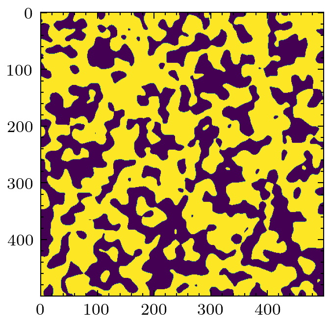
PoreSpy offers several ways to generate artificial images, for quick testing and development of work flows, instead of dealing with reading/writing/storing of large tomograms.

import porespy as ps
import matplotlib.pyplot as plt
im = ps.generators.blobs(shape=[500, 500], porosity=0.6, blobiness=2)
plt.imshow(im)

Applying filters

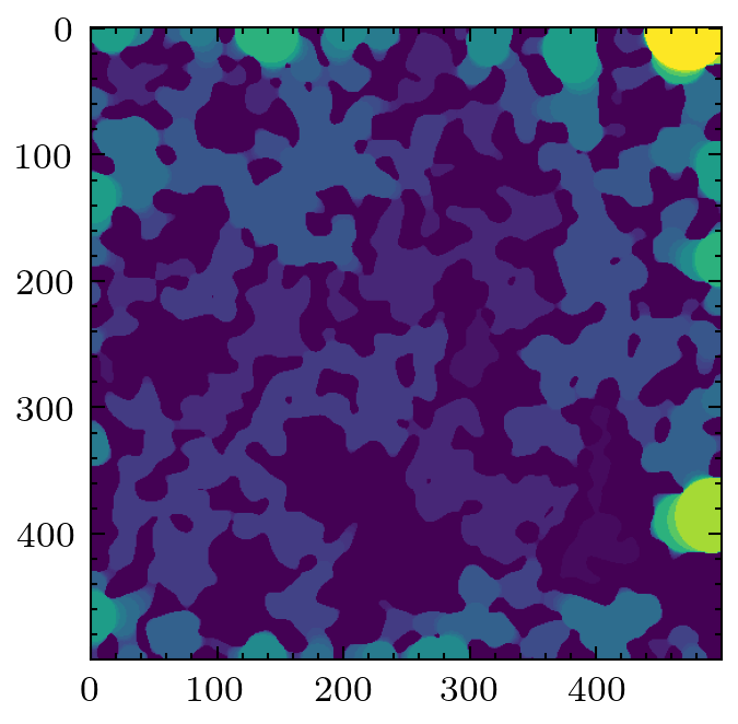
A common filter to apply is the local thickness, which replaces every voxel with the radius of a sphere that overlaps it. Analysis of the histogram of the voxel values provides information about the pore size distribution.

lt = ps.filters.local_thickness(im)
plt.imshow(lt)

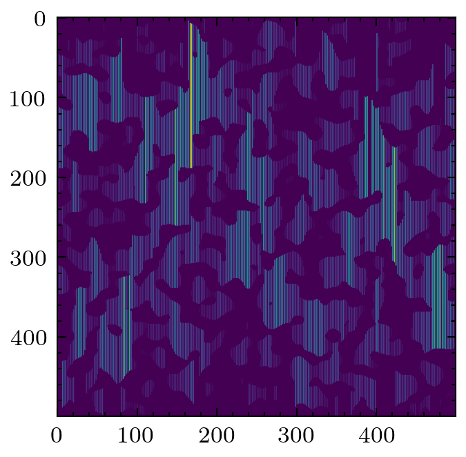
A less common filter is the application of chords that span the pore space in a given direction. It is possible to gain information about anisotropy of the material by looking at the distributions of chords lengths in each principle direction.

cr = ps.filters.apply_chords(im)
cr = ps.filters.flood(cr, mode='size')
plt.imshow(cr)

Calculating metrics

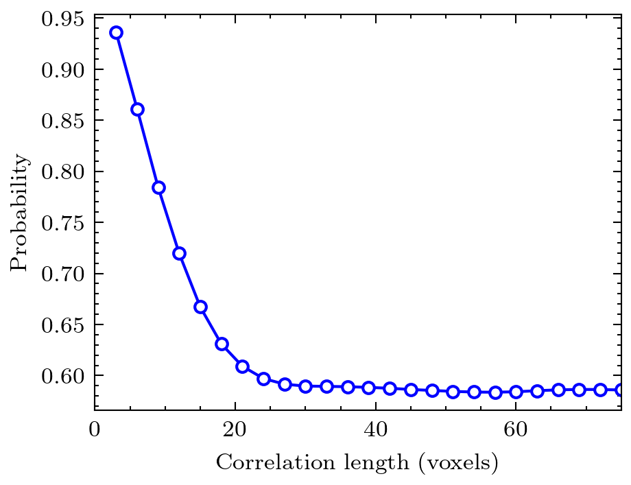
The metrics sub-module contains several common functions that analyze binary tomogram directly. Examples are simple porosity, as well as two-point correlation function.

data = ps.metrics.two_point_correlation_fft(im)
fig = plt.plot(*data, 'bo-')
plt.ylabel('probability')
plt.xlabel('correlation length [voxels]')

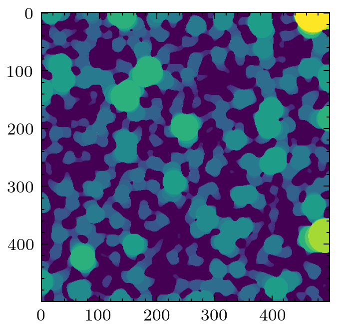
The metrics sub-module also contains a suite of functions that produce plots based on values in images that have passed through a filter, such as local thickness.

mip = ps.filters.porosimetry(im)
data = ps.metrics.pore_size_distribution(mip, log=False)
plt.imshow(mip)
# Now show intrusion curve
plt.plot(data.R, data.cdf, 'bo-')
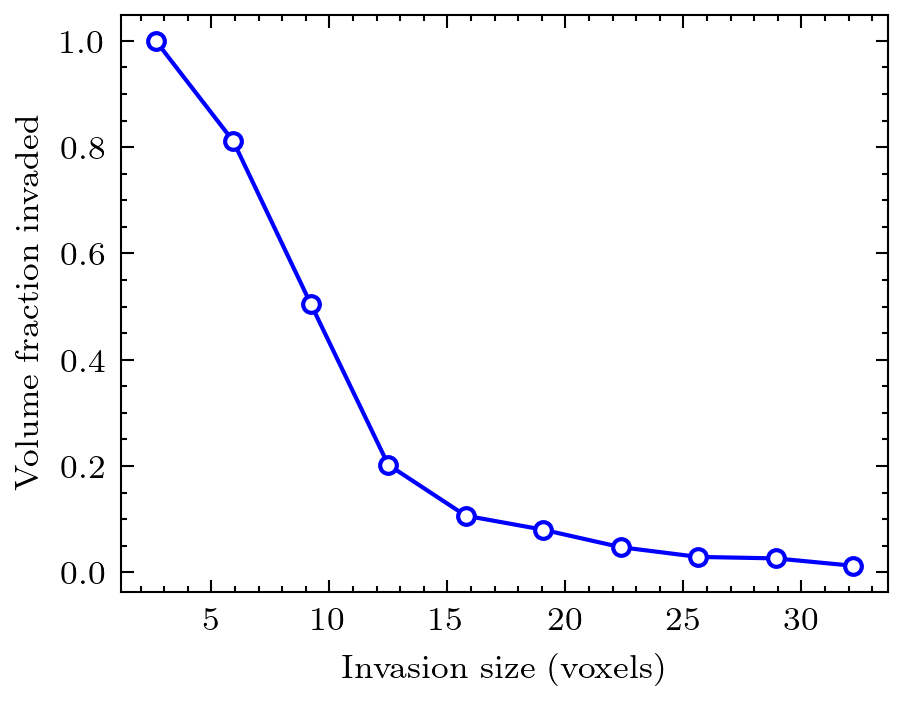
plt.xlabel('invasion size [voxels]')
plt.ylabel('volume fraction invaded [voxels]')