Getting Started

This notebook provides a brief introduction to how PoreSpy works. PoreSpy is designed to use Numpy arrays as images, and more specifically boolean images with True indicating the phase of interest (usually the void phase), so a good understanding of Numpy is required to get the most from PoreSpy.

import porespy as ps
import matplotlib.pyplot as plt
import scipy.ndimage as spim

ps.visualization.set_mpl_style()

[21:16:36] ERROR    PARDISO solver not installed, run `pip install pypardiso`. Otherwise,          _workspace.py:56
                    simulations will be slow. Apple M chips not supported.                                         

Generating Artificial Images

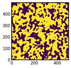
PoreSpy includes a variety of functions for generating artificial image which are useful for prototyping and testing. Below we generate blobs:

im = ps.generators.blobs(shape=[500, 500], porosity=0.6, blobiness=2)

fig, ax = plt.subplots(figsize=[3, 3])
ax.imshow(im);

A full list of generator functions and how to use them can be found here.

Applying Filters

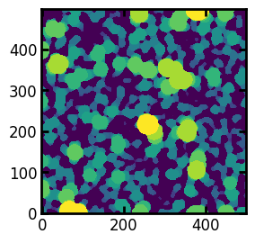
A common filter to apply is the local thickness, which replaces every voxel with the radius of a sphere that overlaps it. Analysis of the histogram of the voxel values provides information about the pore size distribution.

lt = ps.filters.local_thickness(im)

fig, ax = plt.subplots(figsize=[3, 3])
ax.imshow(lt);

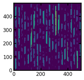
A less common filter is the application of chords that span the pore space in a given direction. It is possible to gain information about anisotropy of the material by looking at the distributions of chords lengths in each principle direction.

cr = ps.filters.apply_chords(im)
labels, N = spim.label(cr)
cr = ps.filters.flood(cr, labels=labels, mode='size')

fig, ax = plt.subplots(figsize=[3, 3])
ax.imshow(cr);

Calculating Metrics

The metrics sub-module contains several common functions that analyze binary tomogram directly. Examples are simple porosity, as well as two-point correlation function.

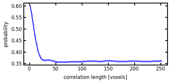
Two-Point Correlation

The metrics sub-module contains several common functions that analyze binary tomogram directly. Examples are simple porosity, as well as two-point correlation function.

data = ps.metrics.two_point_correlation(im)

fig, ax = plt.subplots(figsize=[6, 3])
ax.plot(data.distance, data.probability_scaled, 'bo-', markersize=3)
ax.set_ylabel('probability')
ax.set_xlabel('correlation length [voxels]');

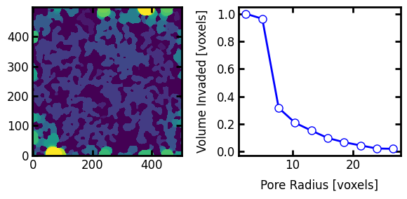
Porosimetry

The metrics sub-module also contains a suite of functions that produce plots based on values in images that have passed through a filter, such as local thickness.

mip = ps.filters.porosimetry(im)
data = ps.metrics.pore_size_distribution(mip, log=False)

fig, ax = plt.subplots(1, 2, figsize=[6, 3])
ax[0].imshow(mip)
# Now show intrusion curve
ax[1].plot(data.R, data.cdf, 'bo-')
ax[1].set_xlabel('Pore Radius [voxels]')
ax[1].set_ylabel('Volume Invaded [voxels]');