SNOW network extraction#
The SNOW algorithm, published in Physical Review E, uses a marker-based watershed segmentation algorithm to partition an image into regions belonging to each pore. The main contribution of the SNOW algorithm is to find a suitable set of initial markers in the image so that the watershed is not over-segmented. SNOW is an acronym for Sub-Network of an Over-segmented Watershed. This code works on both 2D and 3D images. In this example a 2D image will be segmented using the predefined snow function in PoreSpy.
Start by importing the necessary packages:
import matplotlib.pyplot as plt
import numpy as np
import openpnm as op

import porespy as ps

ps.visualization.set_mpl_style()
np.random.seed(10)
[04:04:38] WARNING PARDISO solver not installed on this platform. Simulations will be slow. _workspace.py:56
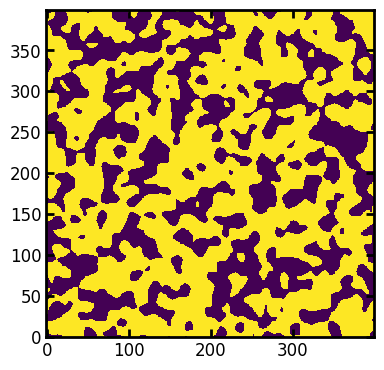
Generate an artificial 2D image for illustration purposes:
im = ps.generators.blobs(shape=[400, 400], porosity=0.6, blobiness=2)
fig, ax = plt.subplots(figsize=(4, 4))
ax.imshow(im);
SNOW is composed of a series of filters, but PoreSpy has a single function that applies all the necessary steps:
snow_output = ps.networks.snow2(im, voxel_size=1)
The snow function returns an object that has a network attribute. This is a dictionary that is suitable for loading into OpenPNM. The best way to get this into OpenPNM is to use the PoreSpy IO class. This splits the data into a network and a geometry:
pn = op.io.network_from_porespy(snow_output.network)
As can be seen by printing the network it contains quite a lot of geometric information:
print(pn)
══════════════════════════════════════════════════════════════════════════════
net : <openpnm.network.Network at 0x7f6555017f20>
――――――――――――――――――――――――――――――――――――――――――――――――――――――――――――――――――――――――――――――
  #  Properties                                                   Valid Values
――――――――――――――――――――――――――――――――――――――――――――――――――――――――――――――――――――――――――――――
  2  throat.conns                                                    283 / 283
  3  pore.coords                                                     261 / 261
  4  pore.region_label                                               261 / 261
  5  pore.phase                                                      261 / 261
  6  throat.phases                                                   283 / 283
  7  pore.region_volume                                              261 / 261
  8  pore.equivalent_diameter                                        261 / 261
  9  pore.local_peak                                                 261 / 261
 10  pore.global_peak                                                261 / 261
 11  pore.geometric_centroid                                         261 / 261
 12  throat.global_peak                                              283 / 283
 13  pore.inscribed_diameter                                         261 / 261
 14  pore.extended_diameter                                          261 / 261
 15  throat.inscribed_diameter                                       283 / 283
 16  throat.total_length                                             283 / 283
 17  throat.direct_length                                            283 / 283
 18  throat.perimeter                                                283 / 283
 19  pore.volume                                                     261 / 261
 20  pore.surface_area                                               261 / 261
 21  throat.cross_sectional_area                                     283 / 283
 22  throat.equivalent_diameter                                      283 / 283
――――――――――――――――――――――――――――――――――――――――――――――――――――――――――――――――――――――――――――――
  #  Labels                                                 Assigned Locations
――――――――――――――――――――――――――――――――――――――――――――――――――――――――――――――――――――――――――――――
  2  pore.all                                                              261
  3  throat.all                                                            283
  4  pore.boundary                                                          43
  5  pore.xmin                                                              12
  6  pore.xmax                                                              11
  7  pore.ymin                                                              10
  8  pore.ymax                                                              10
――――――――――――――――――――――――――――――――――――――――――――――――――――――――――――――――――――――――――――――
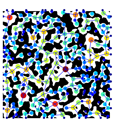
You can also overlay the network on the image natively in porespy. Note that you need to transpose the image using im.T, since imshow uses matrix representation, e.g. a (10, 20)-shaped array is shown as 10 pixels in the y-axis, and 20 pixels in the x-axis.
fig, ax = plt.subplots(figsize=[5, 5])
ax.imshow(im.T, cmap=plt.cm.bone)
op.visualization.plot_coordinates(
    ax=fig,
    network=pn,
    size_by=pn["pore.inscribed_diameter"],
    color_by=pn["pore.inscribed_diameter"],
    markersize=200,
)
op.visualization.plot_connections(network=pn, ax=fig)
ax.axis("off");