MAGNET Network Extraction

The MAGNET algorithm uses the traditional medial axis approach for extracting a network from an image. It makes use of the skeleton by locating pores as the junctions or endpoints of the skeleton.

import matplotlib.pyplot as plt
import numpy as np
import openpnm as op

import porespy as ps

ps.visualization.set_mpl_style()
np.random.seed(10)

[19:36:44] WARNING  PARDISO solver not installed on this platform. Simulations will be slow.       _workspace.py:56

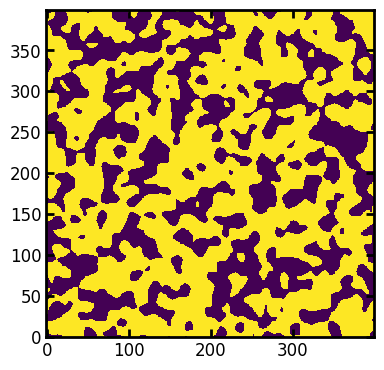
Generate an Image

im = ps.generators.blobs(shape=[400, 400], porosity=0.6, blobiness=2)
fig, ax = plt.subplots(figsize=(4, 4))
ax.imshow(im);

MAGNET uses a series of filters to extract a pore network but porespy has one function that does all this work for you!

magnet_output = ps.networks.magnet(im, voxel_size=1)

The magnet function returns an object that has a network attribute. This is a dictionary that is suitable for loading into OpenPNM. The best way to get this into OpenPNM is to use the PoreSpy IO class. This splits the data into a network and a geometry:

pn = op.io.network_from_porespy(magnet_output.network)

As can be seen by printing the network it contains quite a lot of geometric information:

print(pn)

══════════════════════════════════════════════════════════════════════════════
net : <openpnm.network.Network at 0x7f0745c07d40>
――――――――――――――――――――――――――――――――――――――――――――――――――――――――――――――――――――――――――――――
  #  Properties                                                   Valid Values
――――――――――――――――――――――――――――――――――――――――――――――――――――――――――――――――――――――――――――――
  2  throat.conns                                                    327 / 327
  3  pore.coords                                                     301 / 301
  4  throat.actual_length                                            327 / 327
  5  throat.area                                                     327 / 327
  6  throat.max_diameter                                             327 / 327
  7  throat.min_diameter                                             327 / 327
  8  throat.avg_diameter                                             327 / 327
  9  throat.inscribed_diameter                                       327 / 327
 10  throat.integrated_diameter                                      327 / 327
 11  pore.inscribed_diameter                                         301 / 301
 12  pore.equivalent_diameter                                        301 / 301
 13  pore.index                                                      301 / 301
――――――――――――――――――――――――――――――――――――――――――――――――――――――――――――――――――――――――――――――
  #  Labels                                                 Assigned Locations
――――――――――――――――――――――――――――――――――――――――――――――――――――――――――――――――――――――――――――――
――――――――――――――――――――――――――――――――――――――――――――――――――――――――――――――――――――――――――――――

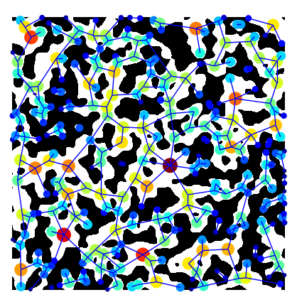
You can also overlay the network on the image natively in porespy. Note that you need to transpose the image using im.T, since imshow uses matrix representation, e.g. a (10, 20)-shaped array is shown as 10 pixels in the y-axis, and 20 pixels in the x-axis.

fig, ax = plt.subplots(figsize=[5, 5])
ax.imshow(im.T, cmap=plt.cm.bone)
op.visualization.plot_coordinates(
    ax=fig,
    network=pn,
    size_by=pn["pore.inscribed_diameter"],
    color_by=pn["pore.inscribed_diameter"],
    markersize=200,
)
op.visualization.plot_connections(network=pn, ax=fig)
ax.axis("off");