Measuring fractal dimension by box-counting

Theory

The term fractal dimension was introduced by Benoit Mandelbrot in 1967 to explain self-similarity of a pattern. A fractal dimension is defined as a ratio of the change in detail to the change in scale. It is used as an index that quantifies the complexity of a fractal pattern.

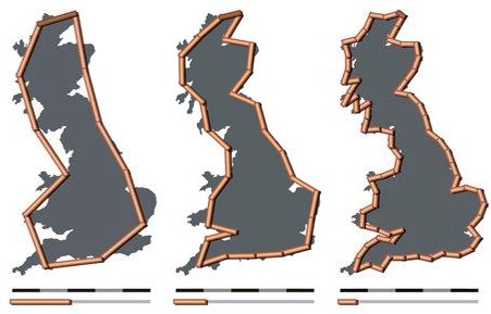
Famously, fractal dimensions have been used to analyze the length of the British coastline. A coastline’s measured length is observed to change depending on the length of the measuring stick used. In 2-D and 3-D, this notion can be extended to the length of a measuring pixel or voxel, respectively.

Box Counting Method

One way to determine fractal dimension of an image is the box counting method. Boxes of various sizes are laid over the image in a fixed grid pattern. The number of boxes that span the edge of the pattern (i.e. partially 1 and partially 0) are tallied as a function of box size. This count is then used to calculate the fractal dimension .

Mathematical Definition

The relationship of a pattern’s fractal dimension and its measuring element can be expressed as:

\[N \propto \frac{1}{D^F}\]

\[F = \lim_{D \to 0} \frac{-log N(D)}{log(D)}\]

where:

• N: number of boxes of side D that span an edge

• D: size of the boxes

• F: fractal dimension

Example

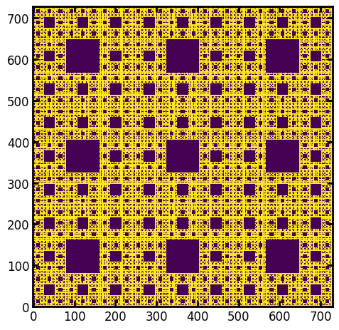
A Sierpinski carpet has a known fractal dimension of 1.8928. Performing the box counting method found its fractal dimension as approximately 1.8 ~ 1.9.

First, import the needed packages.

import matplotlib.pyplot as plt
import porespy as ps
ps.visualization.set_mpl_style()

[19:55:41] ERROR    PARDISO solver not installed, run `pip install pypardiso`. Otherwise,          _workspace.py:56
                    simulations will be slow. Apple M chips not supported.                                         

No module named 'pyedt'

Generate a sierpinski carpet and visualize.

im = ps.generators.sierpinski_foam([3**6, 3**6], n=5, mode=None)
plt.imshow(im);

Finally, apply the box count function and visualize.

data = ps.metrics.boxcount(im)

fig, (ax1, ax2) = plt.subplots(1, 2, figsize=(8, 4))
ax1.set_yscale('log')
ax1.set_xscale('log')
ax1.set_xlabel('box edge length')
ax1.set_ylabel('number of boxes spanning phases')
ax2.set_xlabel('box edge length')
ax2.set_ylabel('slope')
ax2.set_xscale('log')
ax1.plot(data.size, data.count,'-o')
ax2.plot(data.size, data.slope,'-o');

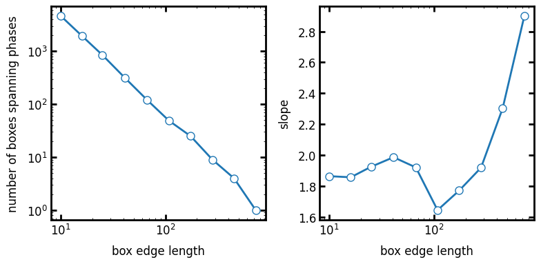
The horizontal portion of the slope vs box edge length curve, between \(10^1\) and \(10^2\) is a flat line with a value of approximately 1.9. Beyond a box edge length of \(10^2\) the analysis becomes impacted by the finite image size so the result begins to diverge.