Using regionprops_3d to analyze properties of each pore

The regionprops function included in Scikit-image is pretty thorough, and the recent version of Scikit-image (>0.14) vastly increase support for 3D images. Nonetheless, there are still a handful of features and properties that are useful for porous media analysis. The regionprops_3d in PoreSpy aims to address thsi need, and it’s use is illustrated here.

import numpy as np
import porespy as ps
import scipy.ndimage as spim
import matplotlib.pyplot as plt
ps.visualization.set_mpl_style()
np.random.seed(1)

[01:05:02] ERROR    PARDISO solver not installed, run `pip install pypardiso`. Otherwise,          _workspace.py:56
                    simulations will be slow. Apple M chips not supported.                                         

Generating a test image

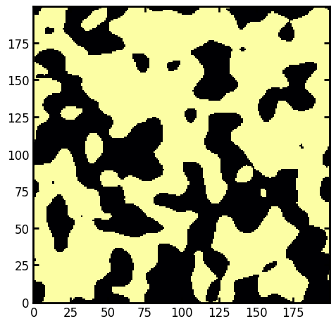
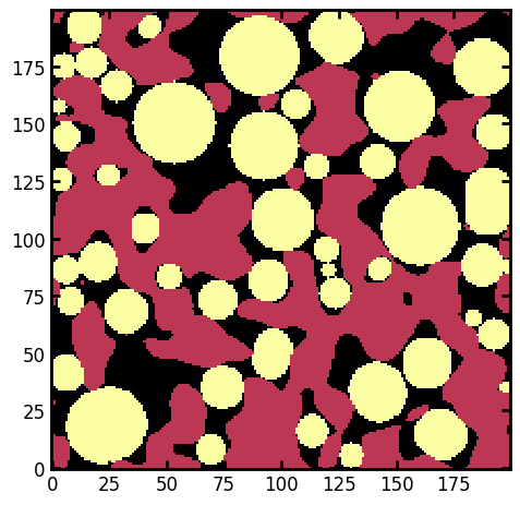
Start by generating a test image using the generators module in PoreSpy.

im = ps.generators.blobs(shape=[200, 200], porosity=0.6, blobiness=1)
fig, ax = plt.subplots()
ax.imshow(im, cmap=plt.cm.inferno);

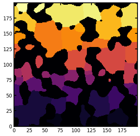
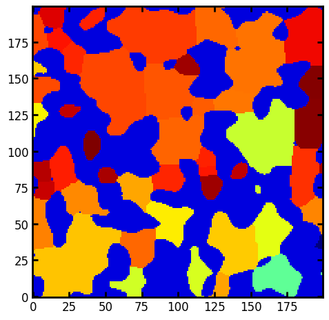
Segementing void space into regions for individual analysis

Next, we need to segment the image into discrete pores, which will become the regions that we analyze. For this purpose we’ll use the SNOW algorithm, which helps to find true local maximums in the distance transform that are used as markers in the watershed segementation.

snow = ps.filters.snow_partitioning(im=im)
regions = snow.regions*snow.im

fig, ax = plt.subplots()
ax.imshow(regions, cmap=plt.cm.inferno);

Applying regionsprops_3d

Now that the void space has been segmented into discrete regions, it’s possible to extract information about each region using regionsprops_3d.

NOTE: PoreSpy calls the Scikit-image regionprops function internally, and uses many of it’s values in subsequent calculations. The result return by regionprops_3d is the same as regionprops of Scikit-image, but with additional information added to each region.

props = ps.metrics.regionprops_3D(regions)

NOTE: The regionprops_3d function in PoreSpy is compatible with the regionsprops function in Scikit-image, which returns the results in a somewhat confusing format. An object is created for each region, and the properites of that region can be accessed as attributes of the object (e.g. obj[10].area). This makes it somewhat annoying, since all the area values cannot be accessed as a single array (PoreSpy has a function to address this, described below), but there is another larger gotcha: Each of the region objects are collected in a list like [obj1, obj2, ...], BUT all regions labelled with 0 are ignored (which is solid phase in this example), so the object located in position 0 of the list corresponds to region 1. Hence, users must be careful to index into the list correctly.

Listing all available properties

Let’s look at some of the properties for the regions, starting by printing a list of all available properties for a given region:

r = props[3]
attrs = [a for a in r.__dir__() if not a.startswith('_')]
print(attrs)

['label', 'slice', 'mask', 'slices', 'volume', 'bbox_volume', 'border', 'dt', 'inscribed_sphere', 'sphericity', 'skeleton', 'surface_area', 'surface_mesh_vertices', 'surface_mesh_simplices', 'convex_volume', 'num_pixels', 'area', 'bbox', 'area_bbox', 'centroid', 'area_convex', 'image_convex', 'coords_scaled', 'coords', 'eccentricity', 'equivalent_diameter_area', 'euler_number', 'extent', 'feret_diameter_max', 'area_filled', 'image_filled', 'image', 'inertia_tensor', 'inertia_tensor_eigvals', 'image_intensity', 'centroid_local', 'intensity_max', 'intensity_mean', 'intensity_min', 'intensity_std', 'axis_major_length', 'axis_minor_length', 'moments', 'moments_central', 'moments_hu', 'moments_normalized', 'orientation', 'perimeter', 'perimeter_crofton', 'solidity', 'centroid_weighted', 'centroid_weighted_local', 'moments_weighted', 'moments_weighted_central', 'moments_weighted_hu', 'moments_weighted_normalized']

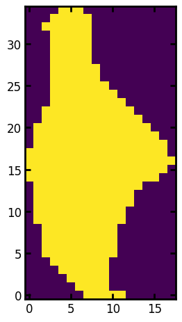
Analyze properties for a single region

Now let’s look at some of the properties for each region, first view image of the region in isolation

fig, ax = plt.subplots()
ax.imshow(r.image);

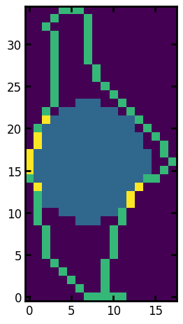
View image of region’s border and largest incribed sphere together.

fig, ax = plt.subplots()
ax.imshow(r.border + 0.5*r.inscribed_sphere);

One of the more interesting properties is the convex image, which is an image of the region with all the depressions in the boundary filled in. This is useful because one can compare it to the actual region and learn about the shape of the region. One such metric is the solidity which is defined as the ratio of pixels in the region to pixels of the convex hull image.

fig, ax = plt.subplots()
ax.imshow(r.image + 1.0*r.convex_image);

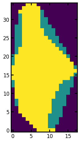
print(f"Solidity: {r.solidity:.3f}")

Solidity: 0.964

Extracting one property for all regions as an array

As mentioned above, the list of objects that are returned by the regionprops_3d funciton is a bit inconvenient for accessing one piece of information for all regions at once. PoreSpy has a function called props_to_DataFrame which helps in this regard by generating a Pandas DataFrame object with all of the key metrics listed as Numpy arrays in each column. Key metrics refers to scalar values like area and solidity.

df = ps.metrics.props_to_DataFrame(props)

/home/runner/work/porespy/porespy/src/porespy/metrics/_regionprops.py:282: FutureWarning: `skeletonize_3d` is deprecated since version 0.23 and will be removed in version 0.25. Use `skimage.morphology.skeletonize` instead.
  return skeletonize_3d(self.mask)

As can be seen above, there are fewer items in this DataFrame than on the regionprops objects. This is because only scalar values are kept (e.g. images are ignored), and some of the metrics were not valid (e.g. intensity_image).

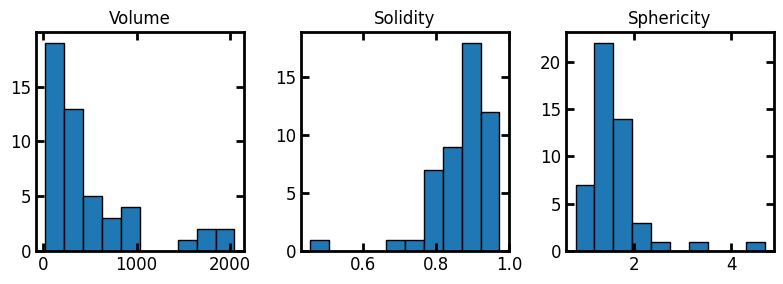
With this DataFrame in hand, we can now look a histograms of various properties:

fig, ax = plt.subplots(1, 3, figsize=(8, 3))
ax[0].hist(df['volume'], edgecolor="k")
ax[1].hist(df['solidity'], edgecolor="k")
ax[2].hist(df['sphericity'], edgecolor="k");
ax[0].set_title("Volume")
ax[1].set_title("Solidity")
ax[2].set_title("Sphericity");

Another useful feature of the Pandas DataFrame is the ability to look at all metrics for a given pore at once, which is done by looking at a single row in all columns:

df.iloc[0]

label                        1.000000
volume                      49.000000
bbox_volume                 55.000000
sphericity                   2.509368
surface_area                25.805790
convex_volume               51.000000
num_pixels                  49.000000
area                        49.000000
area_bbox                   55.000000
area_convex                 51.000000
eccentricity                 0.899545
equivalent_diameter_area     7.898654
euler_number                 1.000000
extent                       0.890909
feret_diameter_max          11.401754
area_filled                 49.000000
axis_major_length           12.017618
axis_minor_length            5.249623
orientation                  1.542041
perimeter                   26.242641
perimeter_crofton           27.561101
solidity                     0.960784
Name: 0, dtype: float64

Creating a composite image of region images

Another useful function available in PoreSpy is prop_to_image, which can create an image from the various subimages available on each region.

# Create an image of maximally inscribed spheres
sph = ps.metrics.prop_to_image(regionprops=props, shape=im.shape, prop='inscribed_sphere')
fig, ax = plt.subplots()
ax.imshow(sph + 0.5*(~im) , cmap=plt.cm.inferno);

Creating a colorized image based on region properties

The prop_to_image function can also accept a scalar property which will result in an image of the regions colorized according to the local value of that property.

# Create an image colorized by solidity
sph = ps.metrics.prop_to_image(regionprops=props, shape=im.shape, prop='solidity')
fig, ax = plt.subplots()
ax.imshow(sph + 0.5*(~im) , cmap=plt.cm.jet);

An interesting result can be seen where the regions at the edges are darker signifying more solidity. This is because the straight edges conform exactly to their convex hulls.