Finding the Tortuosity (\(\tau\)) of an Image Using tortuosity_fd

In this tutorial, we will walk through how to use tortuosity_fd to calculate the tortuosity of an image using a finite difference method. The function takes a binary image to analyze with “True” to indicate the phase of interest as well as the axis along which to find the tortuosity.

Algortihm Description

1. tortuoisty_fd starts by calculating the porosity of the image.
   
   $\( \epsilon_{orginal} = \frac{\sum_{i = 0}^{N_{x}}\sum_{j = 0}^{N_{y}}im_{ij}}{N_{x}\cdot N_{y}} \)$
   
   

2. The second step is to remove non-percolating paths between the inlet and the outlet. This is done by using trim_nonpercolating_paths. The description of this filter can be found here.
   
   

3. The new porosity is calculated after trimming the non-percolating pores using the same equation as step 1.
   
   $\( \epsilon_{eff} = \frac{\sum_{i = 0}^{N_{x}}\sum_{j = 0}^{N_{y}}im_{ij}}{N_{x}\cdot N_{y}} \)$
   
   

4. A cubic network is generated using openpnm and is used as an orthogonal grid.
   
   

5. A dummy phase is created, and openpnm’s Fickian diffusion algorithm (op.algorithms.FickianDiffusion) is applied.
   
   

6. The inlet concentration and throat diffusive conductance are set to 1.0, and the outlet concentration is set to 0.
   
   

7. Using the rate calculated from the Fickian diffusion algorithm, the effective diffusion coefficient is then calculated from the formula:
   
   $\( D_{Eff} = \frac{\dot{\vec{N}} \cdot (L-1)}{A \cdot \Delta C} \)$
   
   

8. The subsequent tortuosity is finally calculated using:
   
   $\(\tau = \frac{D_{AB}}{D_{Eff}} \cdot \varepsilon_{Eff} \)$
   
   

9. All useful results are then compiled into a Results object.

Importing Packages

import matplotlib.pyplot as plt
import porespy as ps
import numpy as np

ps.visualization.set_mpl_style()

[17:49:22] ERROR    PARDISO solver not installed, run `pip install pypardiso`. Otherwise,          _workspace.py:56
                    simulations will be slow. Apple M chips not supported.                                         

Generating the image:

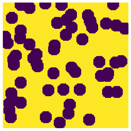
For the purposes of this tutorial, we will generate a 200 x 200 pixel image with a target porosity of 0.65.

np.random.seed(2)
im = ps.generators.overlapping_spheres([200, 200], r=10, porosity=0.65)
fig, ax = plt.subplots()
ax.imshow(im, origin='lower', interpolation='none')
ax.axis(False)

(-0.5, 199.5, -0.5, 199.5)

Running the algorithm

As mentioned at the start of the tutorial, the only two inputs for the function are the image and the axis along which to run the calculation. For the x-axis we assign axis a value of 1 and for the y-axis we assign axis a value of 0.

results = ps.simulations.tortuosity_fd(im=im, axis=1)
print(results)

           WARNING  Found non-percolating regions, were filled to percolate                              _dns.py:74

――――――――――――――――――――――――――――――――――――――――――――――――――――――――――――――――――――――――――――――
Results of tortuosity_fd generated at Tue Apr  9 17:49:23 2024
――――――――――――――――――――――――――――――――――――――――――――――――――――――――――――――――――――――――――――――
im                        Array of size (200, 200)
tortuosity                1.8776173160636371
formation_factor          2.9043927701204795
original_porosity         0.646575
effective_porosity        0.646475
concentration             Array of size (200, 200)
sys                       (<25859x25859 sparse matrix of type '<class 'numpy.float64'>'
	with 124461 stored elements in COOrdinate format>, array([3.8662748, 1.       , 0.       , ..., 0.       , 0.       ,
       0.       ]))
――――――――――――――――――――――――――――――――――――――――――――――――――――――――――――――――――――――――――――――

The function outputs an object with several attributes:

Attribute	Description
tortuosity	The calculated tortuosity is given by the equation: $\(\tau = \frac{D_{AB}}{D_{Eff}} \cdot \varepsilon \)\(<br><br> where \)\varepsilon$ is the effective_porosity
effective_porosity	The effective porosity of the image after removing disconnected voxels
original_porosity	The porosity of the image as inputted
formation_factor	The formation factor is given by the equation: $\(\mathscr{F}=\frac{D_{AB}}{D_{Eff}}\)$
concentration	Returns an image containing the concentration values from the simulation

Calling Values From The Output

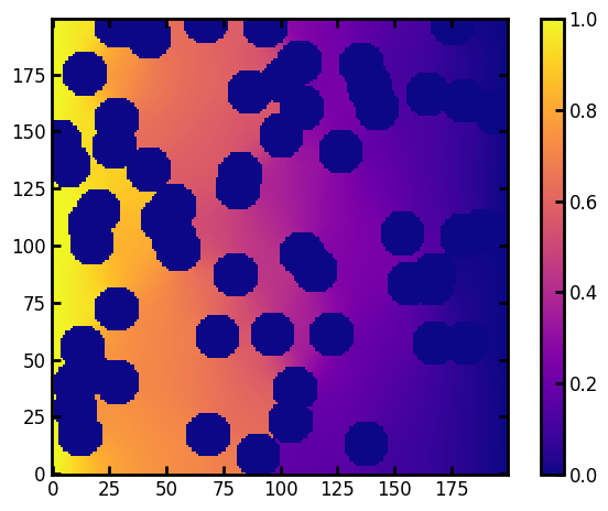
There are a couple ways to call the values from the returned object. The easiest way to call the values is to use object.attribute

plt.imshow(results.concentration,origin='lower', interpolation='none', cmap=plt.cm.plasma)
plt.colorbar()
results.formation_factor

2.9043927701204795