Using AI based diffusive size factors for extracted networks#
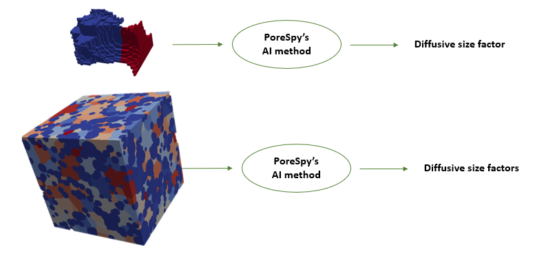
This notebook illustrates the use of the deep learning based diffusive conductance algorithm decribed here. PoreSpy’s diffusive_size_factor_AI includes the steps for predicting the diffusive size factors of the conduit images. Note that the diffusive conductance of the conduits can be then calculated by multiplying the size factor by diffusivity of the phase. The function takes in the images of segmented porous medium and returns an array of diffusive size factors for all conduits in the image. Therefore, the framework can be applied to both one conduit image as well as a segmented image of porous medium:
Trained model and supplementary materials#
To use the diffusive_size_factor_AI, the trained model, and training data distribution are required. The AI model files and additional files used in this example are available here. The folder contains following files:
Trained model weights: This file includes only weights of the deep learning layers. To use this file, the Resnet50 model structure must be built first.
Trained data distribution: This file will be used in denormalizing predicted values based on normalized transform applied on training data. The denormalizing step is included in
diffusive_size_factor_AImethod.Finite difference diffusive conductance: This file is used in this example to compare the prediction results with finite difference method for segmented regions. Note: Finite difference-based size factors can be calculated using PoreSpy’s
diffusive_size_factor_DNSmethod.
Let’s download the tensorflow files required to run this notebook:
try:
    import tensorflow as tf
except ImportError:
    !pip install tensorflow

try:
    import sklearn
except ImportError:
    !pip install scikit-learn

import os

if not os.path.exists("sf-model-lib"):
    !git clone https://github.com/PMEAL/sf-model-lib
2026-03-01 04:04:44.981687: I external/local_xla/xla/tsl/cuda/cudart_stub.cc:31] Could not find cuda drivers on your machine, GPU will not be used.
2026-03-01 04:04:45.032322: I tensorflow/core/platform/cpu_feature_guard.cc:210] This TensorFlow binary is optimized to use available CPU instructions in performance-critical operations.
To enable the following instructions: AVX2 FMA, in other operations, rebuild TensorFlow with the appropriate compiler flags.
2026-03-01 04:04:46.194788: I external/local_xla/xla/tsl/cuda/cudart_stub.cc:31] Could not find cuda drivers on your machine, GPU will not be used.
Also, since the model weights have been stored in chunks, they need to be recombined first:
import importlib

h5tools = importlib.import_module("sf-model-lib.h5tools")
DIR_WEIGHTS = "sf-model-lib/diffusion"
fname_in = [f"{DIR_WEIGHTS}/model_weights_part{j}.h5" for j in [0, 1]]
h5tools.combine(fname_in, fname_out=f"{DIR_WEIGHTS}/model_weights.h5")
Note that to use diffusive_size_factor_AI, Scikit-learn and Tensorflow must be installed. Import necessary packages and the AI model:
import os
import warnings

import h5py
import numpy as np
import openpnm as op
import scipy as sp
from matplotlib import pyplot as plt
from sklearn.metrics import r2_score

import porespy as ps

ps.visualization.set_mpl_style()
warnings.filterwarnings("ignore")
path = "./sf-model-lib/diffusion"
path_train = os.path.join(path, "g_train_original.hdf5")
path_weights = os.path.join(path, "model_weights.h5")
g_train = h5py.File(path_train, "r")["g_train"][()]
model = ps.networks.create_model()
model.load_weights(path_weights)
[04:04:47] WARNING PARDISO solver not installed on this platform. Simulations will be slow. _workspace.py:56
2026-03-01 04:04:48.575287: E external/local_xla/xla/stream_executor/cuda/cuda_platform.cc:51] failed call to cuInit: INTERNAL: CUDA error: Failed call to cuInit: UNKNOWN ERROR (303)
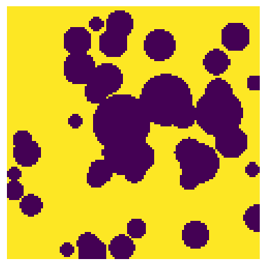
Create test image#
We can create a 3D image using PoreSpy’s poly_disperese_spheres generator:
np.random.seed(17)
shape = [120, 120, 120]
dist = sp.stats.norm(loc=7, scale=5)
im = ps.generators.polydisperse_spheres(shape=shape, porosity=0.7, dist=dist, r_min=7)
fig, ax = plt.subplots(1, 1, figsize=[4, 4])
ax.imshow(im[:, :, 20], origin="lower", interpolation="none")
ax.axis(False);
Extract the network#
We then extract the pore network of the porous medium image using PoreSpy’s snow2 algorithm. snow2 returns the segmented image of the porous medium as well as extracted network data.
snow = ps.networks.snow2(im, boundary_width=0, parallelization=None)
regions = snow.regions
net = snow.network
---------------------------------------------------------------------------
TypeError                                 Traceback (most recent call last)
Cell In[5], line 1
----> 1 snow = ps.networks.snow2(im, boundary_width=0, parallelization=None)
      2 regions = snow.regions
      3 net = snow.network

TypeError: snow2() got an unexpected keyword argument 'parallelization'
Apply diffusive_size_factor_AI#
AI_based diffusive size factors of conduits in the extracted network can then be calculated applying diffusive_size_factor_AI on the segmented regions. We can then define throat.diffusive_size_factor_AI property and assign the predicted size_factor to this property.
conns = net["throat.conns"]
size_factors = ps.networks.diffusive_size_factor_AI(
    regions, model=model, g_train=g_train, throat_conns=conns
)
net["throat.diffusive_size_factor_AI"] = size_factors
47/47 [==============================] - 42s 841ms/step
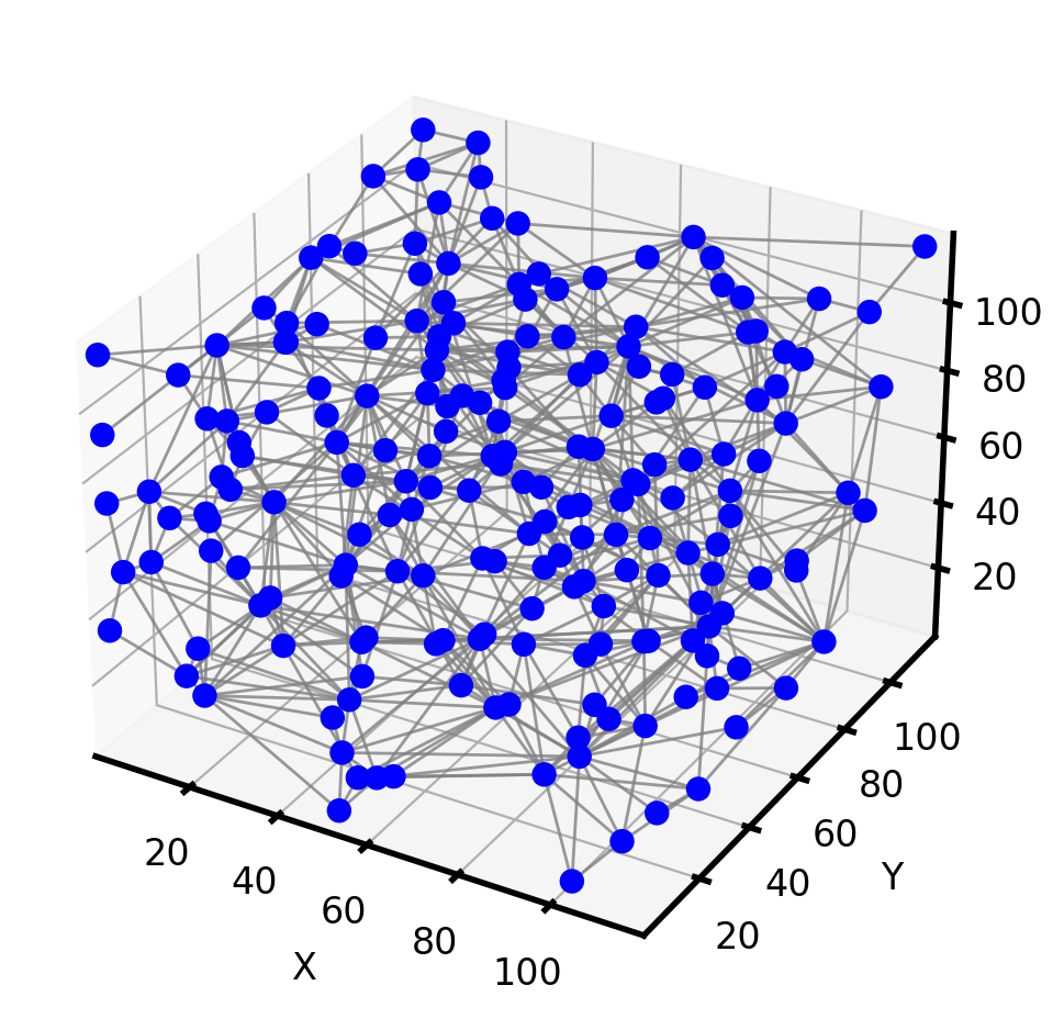
The resulting network can then be imported to OpenPNM for later use such as diffusive mass transport simulations problems. Let’s visualize the network:
pn = op.io.network_from_porespy(net)
fig, ax = plt.subplots(1, 1, figsize=[5, 5])
ax = op.visualization.plot_connections(network=pn, alpha=0.8, color="grey", ax=ax)
ax = op.visualization.plot_coordinates(network=pn, ax=ax, color="b", markersize=50)
Compare with finite difference method#
Now that the extracted network includes AI_based diffusive size factor data, we can use the network to compare the accuracy of diffusive_size_factor_AI, shape factor method,and geometry method (no shape factor) in contrast to finite difference method. Assuming a generic phase with diffusivity of 1, the diffusive conductance of the conduits will be equal to their diffusive size factors. The diffusive conductance of the conduits can be calculated using OpenPNM’s generic_diffusive method. The diffusive conductance of the conduits using shape factor based method assuming cones and cylinders shapes for pores and throats can be calculated as follows:
print(pn)
══════════════════════════════════════════════════════════════════════════════
net : <openpnm.network.Network at 0x7f0256f989a0>
――――――――――――――――――――――――――――――――――――――――――――――――――――――――――――――――――――――――――――――
  #  Properties                                                   Valid Values
――――――――――――――――――――――――――――――――――――――――――――――――――――――――――――――――――――――――――――――
  2  throat.conns                                                    744 / 744
  3  pore.coords                                                     199 / 199
  4  pore.region_label                                               199 / 199
  5  pore.phase                                                      199 / 199
  6  throat.phases                                                   744 / 744
  7  pore.region_volume                                              199 / 199
  8  pore.equivalent_diameter                                        199 / 199
  9  pore.local_peak                                                 199 / 199
 10  pore.global_peak                                                199 / 199
 11  pore.geometric_centroid                                         199 / 199
 12  throat.global_peak                                              744 / 744
 13  pore.inscribed_diameter                                         199 / 199
 14  pore.extended_diameter                                          199 / 199
 15  throat.inscribed_diameter                                       744 / 744
 16  throat.total_length                                             744 / 744
 17  throat.direct_length                                            744 / 744
 18  throat.perimeter                                                744 / 744
 19  pore.volume                                                     199 / 199
 20  pore.surface_area                                               199 / 199
 21  throat.cross_sectional_area                                     744 / 744
 22  throat.equivalent_diameter                                      744 / 744
 23  throat.diffusive_size_factor_AI                                 744 / 744
――――――――――――――――――――――――――――――――――――――――――――――――――――――――――――――――――――――――――――――
  #  Labels                                                 Assigned Locations
――――――――――――――――――――――――――――――――――――――――――――――――――――――――――――――――――――――――――――――
  2  pore.all                                                              199
  3  throat.all                                                            744
――――――――――――――――――――――――――――――――――――――――――――――――――――――――――――――――――――――――――――――
pn["pore.diameter"] = pn["pore.inscribed_diameter"]
pn["throat.diameter"] = pn["throat.inscribed_diameter"]
pn["throat.coords"] = pn["throat.global_peak"]
pn.add_model(
    propname="throat.length", model=op.models.geometry.throat_length.hybrid_cones_and_cylinders
)
pn.add_model(
    propname="throat.diffusive_size_factors",
    model=op.models.geometry.diffusive_size_factors.cones_and_cylinders,
)
phase = op.phase.Phase(network=pn)
phase["pore.diffusivity"] = 1
phase["throat.diffusivity"] = 1
phase.add_model(
    propname="throat.diffusive_conductance",
    model=op.models.physics.diffusive_conductance.generic_diffusive,
)
g_SF = np.copy(phase["throat.diffusive_conductance"])
To find the diffusive conductance of the conduit using geometry method (no shape factor) we assume cylindrical pores and throats:
cn = pn.conns
L1, Lt, L2 = (
    pn["pore.diameter"][cn[:, 0]] / 2,
    pn["throat.length"],
    pn["pore.diameter"][cn[:, 1]] / 2,
)
D1, Dt, D2 = pn["pore.diameter"][cn[:, 0]], pn["throat.diameter"], pn["pore.diameter"][cn[:, 1]]
A1, At, A2 = np.pi * D1**2 / 4, np.pi * Dt**2 / 4, np.pi * D2**2 / 4
g_Geo = 1 / (L1 / A1 + L2 / A2 + Lt / At)
The diffusive conductance of the conduit using AI-based method:
phase.add_model(
    propname="throat.diffusive_conductance",
    model=op.models.physics.diffusive_conductance.generic_diffusive,
    size_factors="throat.diffusive_size_factor_AI",
)
g_AI = np.copy(phase["throat.diffusive_conductance"])
The finite difference-based diffusive size factors were calculated using PoreSpy’s size factor method diffusive_size_factor_DNS. However, due to the long runtime of the DNS function the results were saved in the example data folder and used in this example. The Following code was used to estimate the finite difference-based values using PoreSpy:
g_FD = ps.networks.diffusive_size_factor_DNS(regions, conns)
Now let’s compare the diffusive conductance calculated from geometry-based method, shape factor based-method, and AI-based method with reference finite difference method:
fname = os.path.join(path, "g_finite_difference120-phi7.hdf5")
g_FD = h5py.File(fname, "r")["g_finite_difference"][()]
max_val = np.max([g_FD, g_AI, g_Geo, g_SF])
fig, ax = plt.subplots(1, 3, figsize=[10, 4])

ax[0].plot(g_FD, g_Geo, "*", [0, max_val], [0, max_val], "r")
ax[0].set_xlim([0, max_val])
ax[0].set_ylim([0, max_val])
ax[0].set_xlabel("finite difference $g_d$")
ax[0].set_ylabel("geometry based $g_d$")
ax[0].set_title("$R^2$ = " + str(np.round(r2_score(g_FD, g_Geo), 2)))

ax[1].plot(g_FD, g_SF, "*", [0, max_val], [0, max_val], "r")
ax[1].set_xlim([0, max_val])
ax[1].set_ylim([0, max_val])
ax[1].set_xlabel("finite difference $g_d$")
ax[1].set_ylabel("shape factor based $g_d$")
ax[1].set_title("$R^2$ = " + str(np.round(r2_score(g_FD, g_SF), 2)))

ax[2].plot(g_FD, g_AI, "*", [0, max_val], [0, max_val], "r")
ax[2].set_xlim([0, max_val])
ax[2].set_ylim([0, max_val])
ax[2].set_xlabel("finite difference $g_d$")
ax[2].set_ylabel("AI based $g_d$")
ax[2].set_title(r"$R^2$ = " + str(np.round(r2_score(g_FD, g_AI), 2)));
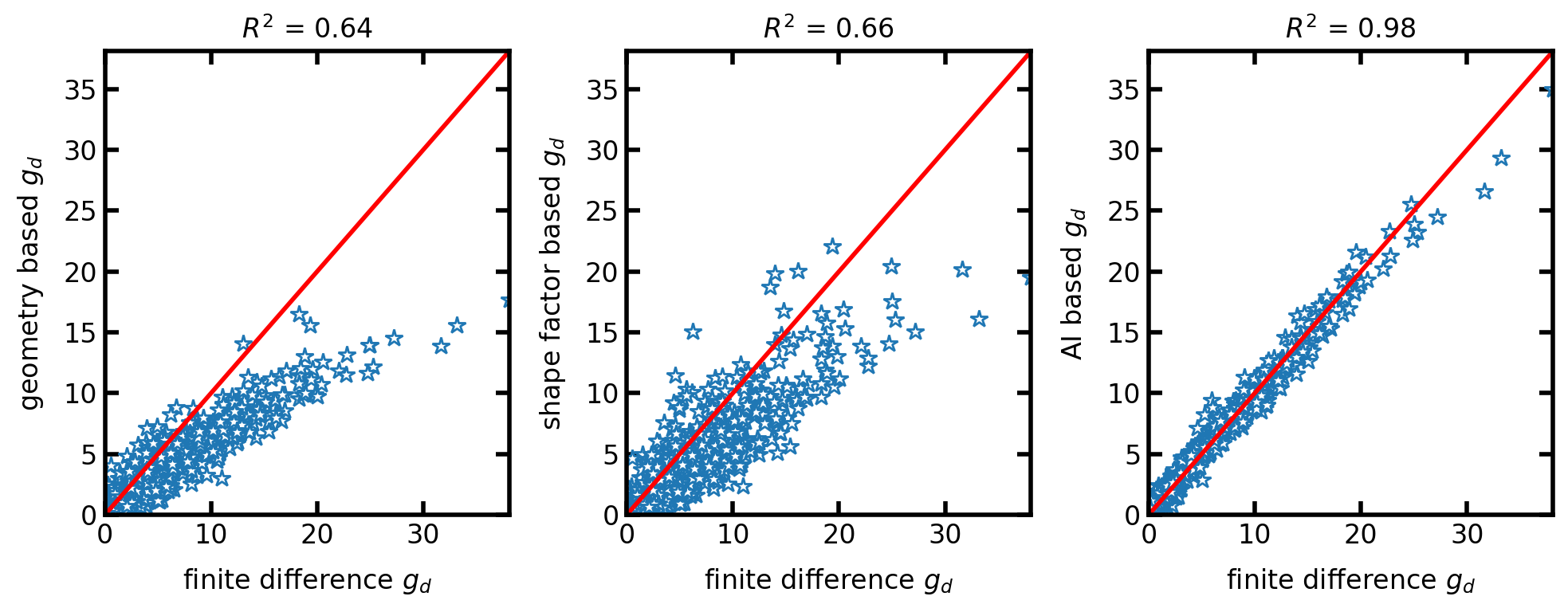
As shown in the scatter plots, the AI-based diffusive conductance method predicts the conductance values with a higher accuracy than geometry-based and shape factor-based methods. A comprehensive comparison between these methods for a large dataset can be found here.