snow2#
The SNOW algorithm uses a standard marker-based watershed segementation function to identify pores. The key to the SNOW algorithm is in how the markers are identified. Finding peaks in the distance transform which truly correspond to pore centers requires several careful steps. Each of these steps can be done manually, but the snow2 function was created to combine them all in a single function for ease of use.
In addition to the original SNOW algorithm, snow2 also incorporates a few new developements such as multiphase extractions and parallelized processing. The new snow2 function also handles boundaries better, and returns a different set of geometrical properties. For instance it no longer returns ‘pore.diameter’, which was an opinionated choice that was not appropriate for every case. Instead it returns several different diameters, like ‘pore.equivalent_diameter’ and ‘pore.inscribed_diameter’, and the user must decide which of these they wish to declare as the offical ‘pore.diameter’.
The snow2 function has quite a few arguments, which will be explored and explained in this example.
import matplotlib.pyplot as plt
import numpy as np
import openpnm as op
import scipy.ndimage as spim
from edt import edt

import porespy as ps
[04:03:25] WARNING PARDISO solver not installed on this platform. Simulations will be slow. _workspace.py:56
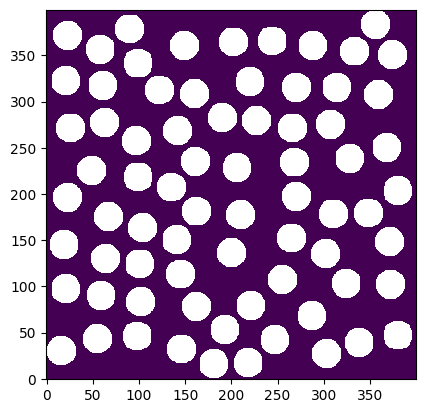
im = ~ps.generators.random_spheres([400, 400], r=15, clearance=5)
ps.imshow(im);
phases#
One of the main features of snow2 is the ability to extract networks from multiple phases simultaneously, and have them be interconnected. This is quite useful for modeling electrochemial devices for instance, since transport occurs in the solid and void phases simultaneously, and the processes are coupled. For a powerful example, see Khan et al. where the transient discharage of a Li-ion battery was modelled using PNMs. Li-ion batteries contain 3 distinct phases: liquid electrolyte, solid active material, and carbonaceous binder.
Note that snow2 does not need to operate on mulitphase phases, only that it can if needed. It accomplishes this flexibility by ignoring all 0’s in the input images, and treating all voxels with values of 1, 2, 3, etc. as distinct phases. Therefore supplying an image of 0’s and 1’s will result in a standard single phase extraction, while supplying an image of 1’s and 2’s will create a dual phase network.
A few additional notes:
It should also be mentioned that the image can contain 0’s as well as values (ie. 1, 2, 3), so can have multiple phases and have some regions ignored
The voxels values do not have be integers or sequential. Each unique numerical value in the image is treated as phase.
Let’s explore this:
im.min()
np.False_
net1 = ps.networks.snow2(phases=im, boundary_width=0)
net2 = ps.networks.snow2(phases=im.astype(int) + 1, boundary_width=0)
The “object” returned by the snow2 function is a dataclass-like object, meaning it has data attached to it as attributes. These attributes are the segmented image called regions, the OpenPNM compatible network called network, and a copy of the input image called phases which will be padded to be the same size as regions if any boundaries were added.
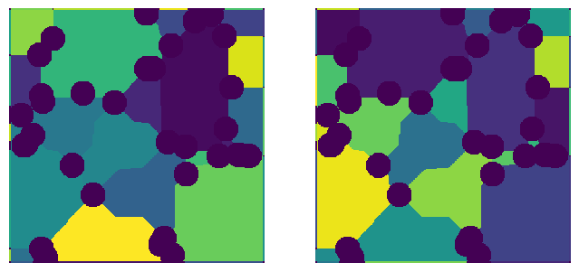
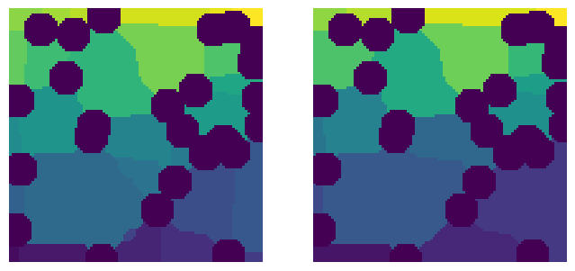
fig, ax = plt.subplots(1, 2, figsize=[12, 6])
ax[0].imshow(net1.regions, origin="lower", interpolation="none")
ax[1].imshow(net2.regions, origin="lower", interpolation="none");
On the left we can see that the spherical particles are all purple, which indicates 0, because they have not been labelled by the function. On the right the particles each have a unique greyscale value because they have been labelled as distinct regions.
The returned objects (net1 and net2) also contain the pore networks, in OpenPNM format. We can overlay these networks with the above images. Let’s start with the single phase network:
pn1 = op.io.network_from_porespy(net1.network)
ax = op.visualization.plot_connections(pn1, c="k")
ax = op.visualization.plot_coordinates(pn1, markersize=50, ax=ax)
fig, ax = plt.gcf(), plt.gca()
ax.imshow(net1.regions.T)
ax.axis(False);

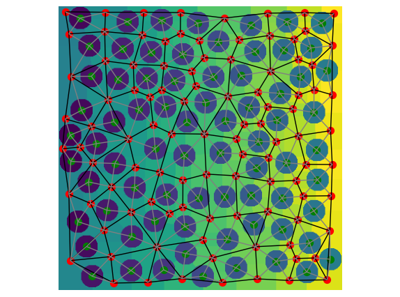
The image needed to be rotated so that the x and y directions lined up with the OpenPNM network. The agreement between the image and network is pretty good. Clearly the the red pore centers lie within each labelled regions and the black throat connections follow the topology quite well.
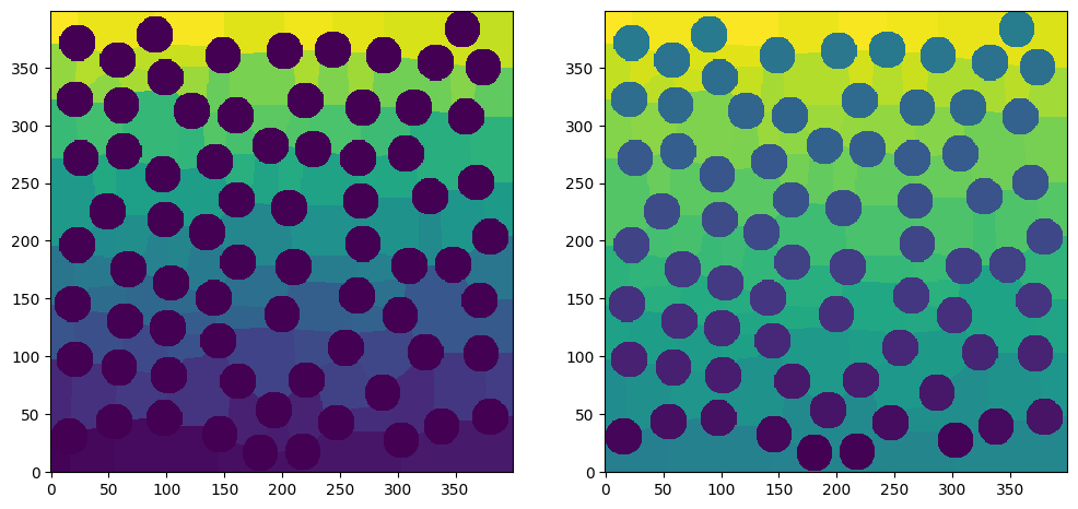
Now let’s do the same for the multiphase network:
pn2 = op.io.network_from_porespy(net2.network)
ax = op.visualization.plot_connections(pn2, c="k")
ax = op.visualization.plot_coordinates(pn2, markersize=50, ax=ax)
fig, ax = plt.gcf(), plt.gca()
ax.imshow(net2.regions.T)
ax.axis(False);
The above shows the additional network comprised of the solids (although they don’t actually connect in this 2D example) as well as the void-solid connections. We can improve this plot by coloring the different types of pores and throats differently. If we print pn2 we can see that snow2 has created some labels for us, by assuming phase names of “phase1” and “phase2”.
print(pn2)
══════════════════════════════════════════════════════════════════════════════
net : <openpnm.network.Network at 0x7f7b14810eb0>
――――――――――――――――――――――――――――――――――――――――――――――――――――――――――――――――――――――――――――――
  #  Properties                                                   Valid Values
――――――――――――――――――――――――――――――――――――――――――――――――――――――――――――――――――――――――――――――
  2  throat.conns                                                    486 / 486
  3  pore.coords                                                     172 / 172
  4  pore.region_label                                               172 / 172
  5  pore.phase                                                      172 / 172
  6  throat.phases                                                   486 / 486
  7  pore.region_volume                                              172 / 172
  8  pore.equivalent_diameter                                        172 / 172
  9  pore.local_peak                                                 172 / 172
 10  pore.global_peak                                                172 / 172
 11  pore.geometric_centroid                                         172 / 172
 12  throat.global_peak                                              486 / 486
 13  pore.inscribed_diameter                                         172 / 172
 14  pore.extended_diameter                                          172 / 172
 15  throat.inscribed_diameter                                       486 / 486
 16  throat.total_length                                             486 / 486
 17  throat.direct_length                                            486 / 486
 18  throat.perimeter                                                486 / 486
 19  pore.volume                                                     172 / 172
 20  pore.surface_area                                               172 / 172
 21  throat.cross_sectional_area                                     486 / 486
 22  throat.equivalent_diameter                                      486 / 486
――――――――――――――――――――――――――――――――――――――――――――――――――――――――――――――――――――――――――――――
  #  Labels                                                 Assigned Locations
――――――――――――――――――――――――――――――――――――――――――――――――――――――――――――――――――――――――――――――
  2  pore.all                                                              172
  3  throat.all                                                            486
  4  pore.phase1                                                            73
  5  throat.phase1_phase2                                                  315
  6  pore.phase2                                                            99
  7  throat.phase2_phase1                                                  315
  8  throat.phase2_phase2                                                  171
――――――――――――――――――――――――――――――――――――――――――――――――――――――――――――――――――――――――――――――
ax = op.visualization.plot_connections(pn2, throats=pn2["throat.phase2_phase2"], c="k")
ax = op.visualization.plot_connections(
    pn2, throats=pn2["throat.phase2_phase1"], c="grey", ax=ax
)
ax = op.visualization.plot_coordinates(
    pn2, pores=pn2["pore.phase2"], c="r", markersize=50, ax=ax
)
ax = op.visualization.plot_coordinates(
    pn2, pores=pn2["pore.phase1"], c="g", markersize=50, ax=ax
)
fig, ax = plt.gcf(), plt.gca()
ax.imshow(net2.regions.T)
ax.axis(False);
Now can see the particles are indicated by a green marker, the void pores by a red marker, the solid-void interconnections are in grey, and the void-void throats are black.
phase_alias#
In the previous section the default phase names created by snow2 were the uncreative “phase1” and “phase2”. The snow2 function allows for these to be given more desriptive names. This is done by supplying a dictionary with the voxels value as the key and the desired phase name as the value.
net3 = ps.networks.snow2(
    phases=im.astype(int) + 1, phase_alias={1: "solid", 2: "void"}, boundary_width=0
)
pn3 = op.io.network_from_porespy(net3.network)
print(pn3)
══════════════════════════════════════════════════════════════════════════════
net : <openpnm.network.Network at 0x7f7b14a78550>
――――――――――――――――――――――――――――――――――――――――――――――――――――――――――――――――――――――――――――――
  #  Properties                                                   Valid Values
――――――――――――――――――――――――――――――――――――――――――――――――――――――――――――――――――――――――――――――
  2  throat.conns                                                    486 / 486
  3  pore.coords                                                     172 / 172
  4  pore.region_label                                               172 / 172
  5  pore.phase                                                      172 / 172
  6  throat.phases                                                   486 / 486
  7  pore.region_volume                                              172 / 172
  8  pore.equivalent_diameter                                        172 / 172
  9  pore.local_peak                                                 172 / 172
 10  pore.global_peak                                                172 / 172
 11  pore.geometric_centroid                                         172 / 172
 12  throat.global_peak                                              486 / 486
 13  pore.inscribed_diameter                                         172 / 172
 14  pore.extended_diameter                                          172 / 172
 15  throat.inscribed_diameter                                       486 / 486
 16  throat.total_length                                             486 / 486
 17  throat.direct_length                                            486 / 486
 18  throat.perimeter                                                486 / 486
 19  pore.volume                                                     172 / 172
 20  pore.surface_area                                               172 / 172
 21  throat.cross_sectional_area                                     486 / 486
 22  throat.equivalent_diameter                                      486 / 486
――――――――――――――――――――――――――――――――――――――――――――――――――――――――――――――――――――――――――――――
  #  Labels                                                 Assigned Locations
――――――――――――――――――――――――――――――――――――――――――――――――――――――――――――――――――――――――――――――
  2  pore.all                                                              172
  3  throat.all                                                            486
  4  pore.solid                                                             73
  5  throat.solid_void                                                     315
  6  pore.void                                                              99
  7  throat.void_solid                                                     315
  8  throat.void_void                                                      171
――――――――――――――――――――――――――――――――――――――――――――――――――――――――――――――――――――――――――――――
Now we can see that the phases are named using our preferred nomenclature of “solid” and “void”. This is helpful if you have several phases like “electrolyte”, “binder”, “particles” for instance.
boundary_width#
Adding pores (or more generally nodes) on the boundaries of images is helpful when conducting transport simulations. Without boundary pores then boundary condtions must be applied to internal pores which are (a) hard to identify clearly and (b) make it impossible to know the exact length of the domain.
Note that boundary nodes are not physical and thus their sizes are ficticious. This can cause problems when computing the transport conductance for these nodes, so care must be taken.
The boundary_width argument was designed to work analogously to the numpy.pad function. You can specify different paddings along each axis and also along each face. For instance, here are some options (for a 2D image):
[0, 3]: 3 voxels only applied to the y-axis.[0, [0, 3]]: 3 voxels only applied to the end of y-axis.[0, [3, 0]]: 3 voxels only applied to the beginning of y-axis.
im = ps.generators.blobs([400, 400], porosity=0.6)
a = ps.networks.snow2(im, boundary_width=[[5, 0], 10])
fig, ax = plt.subplots(figsize=[6, 6])
ax.imshow(a.regions, origin="lower", interpolation="none")
ax.axis(False);
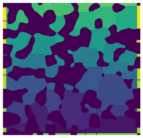
A few things to note:
The image contains regions on the left, right and bottom faces, which are added by padding the image after the segmentation was applied, then incrementing labels the padded regions so their labels are greater than any inside the original image.
These new regions are then treated like a normal region when the network topology and geometry is extracted.
The width of each boundary region is nearly the same as the corresponding internal regions, but they are only a few voxels thick (in this case because we specified 5 or 10). This means that the value of ‘pore.inscribed’ sphere for this regions will almost all be 5 or 10 voxels.
The solid touching the boundaries creates gaps in the boundary regions.
Two boundary regions neighboring each other are separated by 2 voxels. This prevents them from being considered as connected during the topology extraction stage.
The top and bottom of the image do not have any boundaries because we set the widths to 0 on this axis.
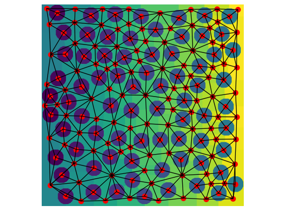
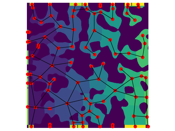
It is instructive to visualize the network over the image to see how the boundary pores work:
pn = op.io.network_from_porespy(a.network)
ax = op.visualization.plot_connections(pn, c="k")
ax = op.visualization.plot_coordinates(pn, markersize=50, ax=ax)
fig, ax = plt.gcf(), plt.gca()
ax.imshow(a.regions.T)
ax.axis(False);
accuracy#
This argument can either take the value of 'high' or 'standard', with standard being the default. It is not recommended to use 'high' since this uses some rather slow functions to measure the surface areas and perimeters. The increase in accuracy is basically futile since (a) the image has already been reduced to a coarse voxelization and (b) the pore network abstraction discards information about the actual microstructure in exchange for speed, so spending ages on the extraction step would undermine this purpose.
voxel_size#
This is the voxel size of the image, as in the length of one side of a voxel. Typical microtomography images are in the range of 1-5 um per voxel. NanoCT can be as low as 16 nm per voxel. FIB-SEM might be 4 nm per voxel. Note that all properties returned from the snow2 function, like ‘pore.volume’ will be in the same units are this value. It is strongly recommended to use SI, which is assumed in OpenPNM for most of the fluid property calculations.
sigma and r_max#
These values are passed on to the gaussian_blur and find_peaks functions.
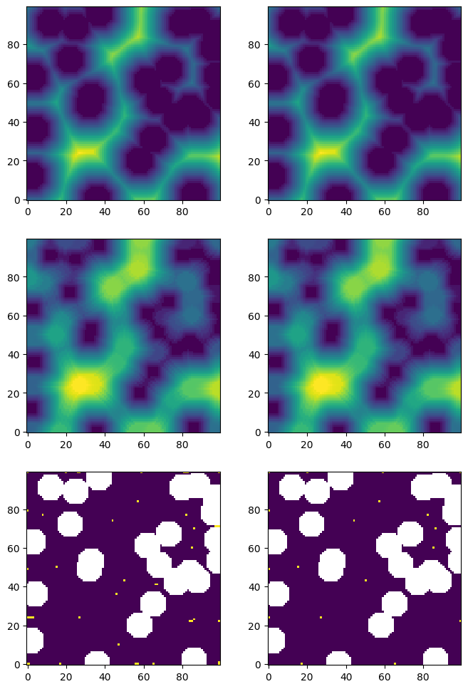
The gaussian_blur is applied to the distance transfrom, which as discussed in the original snow paper is a very effective way to reduce the number of incorrect peaks that are found in the subsequent steps. A value of sigma=0.4 is the default.
The find_peaks function applies a maximum filter to the distance transform, which replaces each voxel with the maximum it finds with the specified neighborhood. It then looks for voxels that are the same between the filtered image and the original distance transform. Only voxels that are local maximas will be the same between the images.
The following code block illustrates the impact of applying the gaussian_blur filter on finding peaks.
np.random.seed(13)
im = ps.generators.overlapping_spheres([100, 100], r=7, porosity=0.7)
dt = edt(im)
mx1 = spim.maximum_filter(dt, footprint=ps.tools.ps_disk(r=4, smooth=False))
pk1 = dt == mx1
dt_blur = spim.gaussian_filter(dt, sigma=0.4)
mx2 = spim.maximum_filter(dt_blur, footprint=ps.tools.ps_disk(r=4, smooth=False))
pk2 = dt_blur == mx2
fig, ax = plt.subplots(3, 2, figsize=[8, 12])
ax[0][0].imshow(dt, origin="lower", interpolation="none")
ax[1][0].imshow(mx1, origin="lower", interpolation="none")
ax[2][0].imshow(pk1 / im, origin="lower", interpolation="none")
ax[0][1].imshow(dt_blur, origin="lower", interpolation="none")
ax[1][1].imshow(mx2, origin="lower", interpolation="none")
ax[2][1].imshow(pk2 / im, origin="lower", interpolation="none");
peaks#
Because finding correct peaks is such an important part marker-based watershed segmentationa, and therefore of snow2, it is possible to supply custom peaks found using any desired process. Obviously, if this is provided then sigma and r_max are ignored.
Let’s use the two sets of peaks found above:
net1 = ps.networks.snow2(phases=im, boundary_width=0, peaks=pk1)
net2 = ps.networks.snow2(phases=im, boundary_width=0, peaks=pk2)
fig, ax = plt.subplots(1, 2, figsize=[8, 4])
ax[0].imshow(net1.regions, origin="lower", interpolation="none")
ax[1].imshow(net2.regions, origin="lower", interpolation="none")
ax[0].axis(False)
ax[1].axis(False);
Clearly the image on the left is ‘over segmented’ while the image on the right seems to have identified the pores nearly perfectly, even without subsequent processing of the peaks that normally occur in snow2 like trim_saddle_points and trim_nearby_peaks.
parallelization#
The watershed function was identified as the bottleneck of the entire process, especially as images grew in size. Parallelization of the watershed function had not be throughly investigated in the literature, so Khan et al developed a basic protocol for dividing the image into chunks and processing each in parallel. The main challenge with this approach was ensuring sufficient overlap was allowed to prevent any artifacts, while not being overly conservative since large overlaps undermine the speedup obtained by parallelization. The parallelization if accomplished by dask which makes it trivial to dispatch duplicate jobs to different cores.
The snow2 function can optionally parallelize the watershed step. It calls porespy.filters.snow_partitioning_parallel behind the scenes, but this function requires several arguments. Instead of complicating the snow2 function signature, we instead chose to accept a dict of arguments and values which are then passed on. These are:
divs: The number of chunks to divide the image into. A value of 2 means the image is divided in hald along each axis, for a total of 8 chunks in a 3D image. It’s possible to specify a different number of divisions in each direction, likedivs=[2, 2, 1]. This could be useful if the image to be processed is very narrow in one direction, such as a piece of fibrous electrode.overlap: This controls the amount of overlap between each chunk in voxels. SpecifyingNone(the default) means that the algorithm finds the overlap automatically. Khan el al found that using the maximum of the distance tranform was suitable.cores: This controls the number of cores to use when processing the chunks. If not provided then all cores will be used. This may be problematic on computers without a large amount of RAM since each process will consume some RAM. In these cases in may be beneficial to set cores to a small number and simply wait longer for the result.
If parallel_kw=None then no parallelization is applied, while if parallel_kw={} then the default arguments of the snow_partitioning_parallel function are used.
In the following code block, the parallelization option is demonstrated with an overlap that is too small, resulting in a noticable artifacts in the center sectionof the watershed segmentation, where the divsions were located. For comparison, the same image is processed with the default overlap.
np.random.seed(0)
im = ps.generators.overlapping_spheres([400, 400], r=20, porosity=0.8)
parallel_kw = {"cores": 1, "divs": [2, 2], "overlap": 1}
net1 = ps.networks.snow2(phases=im, parallel_kw=parallel_kw)
parallel_kw = {"cores": 1, "divs": [2, 2], "overlap": None}
net2 = ps.networks.snow2(phases=im, parallel_kw=parallel_kw)
fig, ax = plt.subplots(1, 2, figsize=[8, 4])
temp = ps.tools.randomize_colors(net1.regions)
ax[0].imshow(temp, origin="lower", interpolation="none")
ax[0].axis(False)
temp = ps.tools.randomize_colors(net2.regions)
ax[1].imshow(temp, origin="lower", interpolation="none")
ax[1].axis(False);