Local thickness

This example explains how to use the local_thickness filter to get information about the pore size distribution from an image. The local thickness is probably the closest you can get to an actual pore size distribution. Unlike porosimetry experiments or simulations, it is unaffected by artifacts such as edge effects and access limitations. The implementation in PoreSpy is slightly different than the common approach done in ImageJ, as will be explained below.

import numpy as np
import porespy as ps
import scipy.ndimage as spim
import matplotlib.pyplot as plt
ps.visualization.set_mpl_style()

[17:43:48] ERROR    PARDISO solver not installed, run `pip install pypardiso`. Otherwise,          _workspace.py:56
                    simulations will be slow. Apple M chips not supported.                                         

Generate Test Image

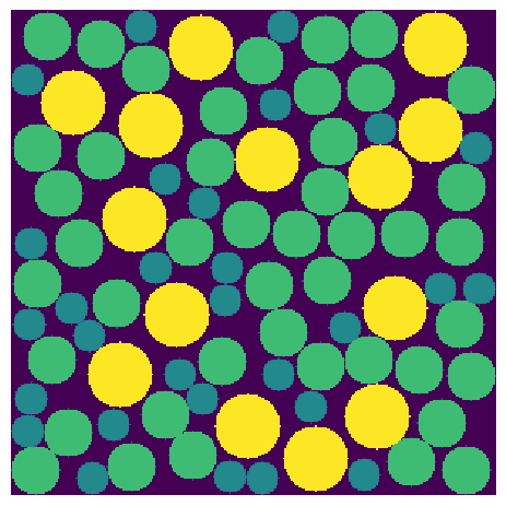
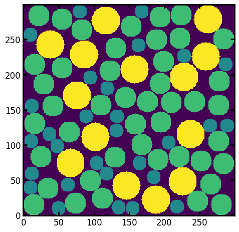
Start by generating an image. We’ll use the RSA generator for fun:

im = np.ones([300, 300])
im = ps.generators.random_spheres(im=im, r=20, phi=0.2, smooth=False)
im = ps.generators.random_spheres(im=im, r=15, phi=0.4, smooth=False)
im = ps.generators.random_spheres(im=im, r=10, phi=0.6, smooth=False)
im = im == 0
fig, ax = plt.subplots()
ax.imshow(im, interpolation='none', origin='lower')
ax.axis(False);

Apply Local Thickness Filter

The local thickness filter is called by simply passing in the image. Like all filters in PoreSpy it is applied to the foreground, indicated by 1’s or True:

thk = ps.filters.local_thickness(~im, mode='dt')
fig, ax = plt.subplots()
ax.imshow(thk, interpolation='none', origin='lower', cmap=plt.cm.jet)
ax.axis(False);

Extracting PSD as a Histogram

Obtaining pore size distribution information from this image requires obtaining a histogram of voxel values. A function in the metrics module does this for us:

psd = ps.metrics.pore_size_distribution(im=thk)

This function, like many of the functions in the metrics module, returns several arrays lumped together on a single object. The advantage of this is that each array can be accessed by name as attributes, such as psd.pdf. To see all the available attributes (i.e. arrays) use the autocomplete function if your IDE supports it, or just print it as follows:

print(psd)

――――――――――――――――――――――――――――――――――――――――――――――――――――――――――――――――――――――――――――――
Results of pore_size_distribution generated at Tue Apr  9 17:43:49 2024
――――――――――――――――――――――――――――――――――――――――――――――――――――――――――――――――――――――――――――――
LogR                      Array of size (10,)
pdf                       Array of size (10,)
cdf                       Array of size (10,)
satn                      Array of size (10,)
bin_centers               Array of size (10,)
bin_edges                 Array of size (11,)
bin_widths                Array of size (10,)
――――――――――――――――――――――――――――――――――――――――――――――――――――――――――――――――――――――――――――――

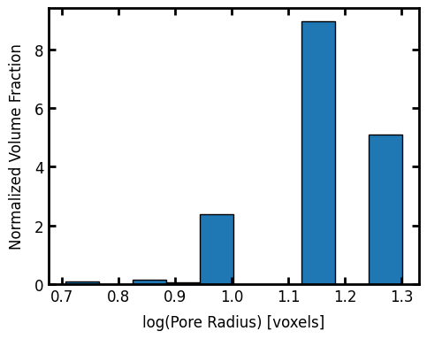
Let’s plot a pore-size distribution histogram:

fig, ax = plt.subplots(figsize=(5, 4))
ax.set_xlabel('log(Pore Radius) [voxels]')
ax.set_ylabel('Normalized Volume Fraction')
ax.bar(x=psd.LogR, height=psd.pdf, width=psd.bin_widths, edgecolor='k');

PoreSpy Implementation

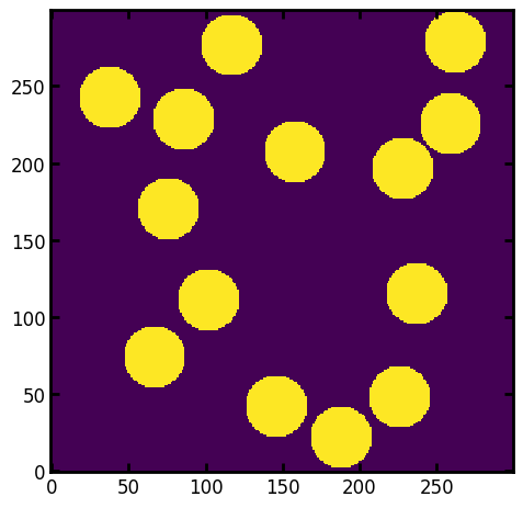
The local_thickness filter in PoreSpy is implemented differently that the normal approach such as the ImageJ plugin, though the end result is comparible though not identical.

In our approach, we use a form of image dilation and erosion. We start with a large spherical structuring element, and note all the places where this fits in the pore space. This gives a result like that below for a structuring element of radius R=10:

R = 10 
strel = ps.tools.ps_disk(R)
im_temp = spim.binary_opening(~im, structure=strel)
fig, ax = plt.subplots()
ax.imshow(im_temp*2.0 + ~im, interpolation='none', origin='lower');

The key is to make a master array containing the numerical value of the largest sphere that covers each voxel. We’ll initialize a new array with the current locations where R=10 fits:

im_result = im_temp*R

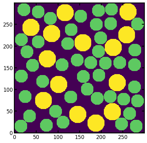
Now this is repeated for a range of decreasing structuring element sizes. For illustration, do R = 8:

R = 8
strel = ps.tools.ps_disk(R)
im_temp = spim.binary_opening(~im, structure=strel)

This new image must be added to the im_result array, but only in places that were not filled at any larger radius. This is done using boolean logic as follows:

im_result[(im_result == 0)*im_temp] = R

There are now 2 values in the im_results array indicating the locations where the structuring element of size 10 fits, and where size 8 fit on the subsequent step:

fig, ax = plt.subplots()
ax.imshow(im_result - im*1.5, interpolation='none', origin='lower');

The procedure is then repeated for smaller structuring elements down to R = 1. It’s possible to specify which sizes are used, but by default all integers between \(R_{max}\) and 1. This yields the image showed above:

fig, ax = plt.subplots()
ax.imshow(thk, cmap=plt.cm.jet, interpolation='none', origin='lower');