satn_to_panels

Produces a set of images with each panel containing one saturation. This method can be applied for visualizing image-based invasion percolation algorithm ibip filter.

import matplotlib.pyplot as plt
import numpy as np

import porespy as ps

ps.visualization.set_mpl_style()

im

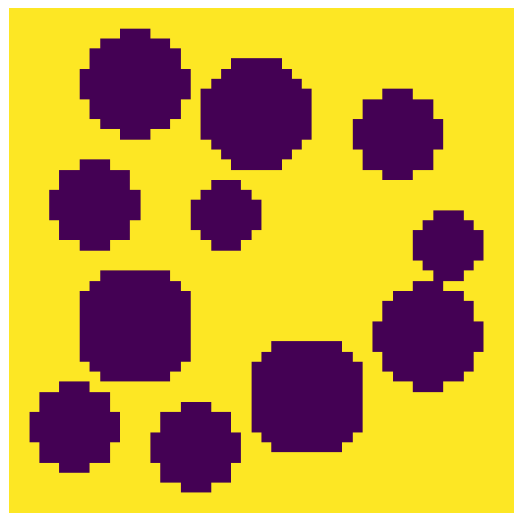
The input image is a Boolean image True values indicating the void voxels and False for solid. Let’s create a test image:

np.random.seed(10)
im = ~ps.generators.random_spheres(shape=[50, 50, 50], r=5)
fig, ax = plt.subplots(1, 1, figsize=[6, 6])
ax.imshow(im[:, :, 20], origin="lower", interpolation="none")
ax.axis(False);

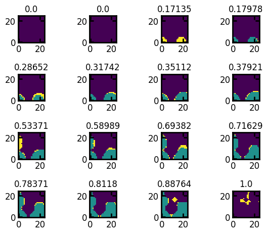
satn

The saturation image can be generated from any of the image-based invasion simulations, like ibip or ibop, the the result can be converted to saturaiton using seq_to_satn. The satn is the image of porous material where each voxel indicates the global saturation at which it was invaded. Voxels with 0 values indicate solid and and -1 indicate uninvaded. As the image is large, we will be visualizing a section of the image: Note that the regions that were uninvaded at sat=0.7 are now invaded at sat=0.75 and remaining regions are invaded at sat=1:

out = ps.simulations.drainage(im=im)
satn = out.im_snwp
fig, ax = ps.visualization.satn_to_panels(satn[:25, :25, 10], im[:25, :25, 10])

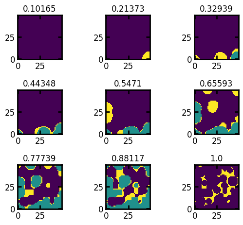
bins

Indicates for which saturations images should be made. By default 16 saturation values in the image are used. To visualize the image for a list of equally space values between 0 and 1, an int value can be passed as the input (the number of saturation points between [0,1]).

fig, ax = ps.visualization.satn_to_panels(satn, im, bins=9)

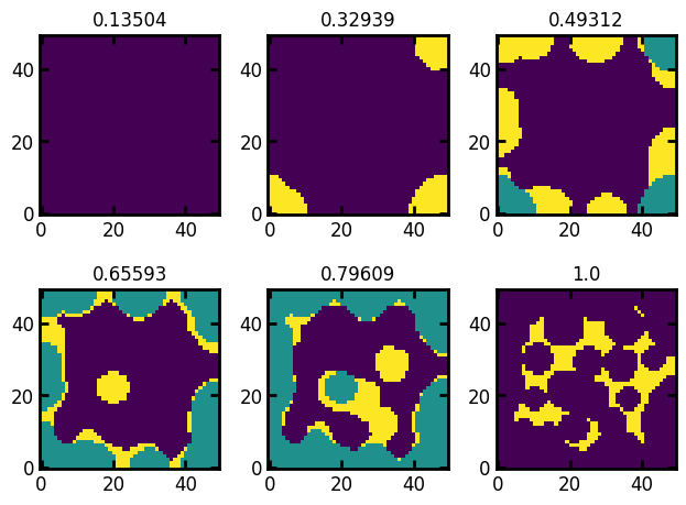
axis

If the image is 2D this variable is ignored. If the image is 3D, a 2D image is extracted at the specified slice taken along this axis. By default axis=0 indicating the slice is extracted at x axis. Let’s extract the slices at y axis (because slice is not passed as the input, the default slice is at the mid-point of the axis):

fig, ax = ps.visualization.satn_to_panels(satn, im, bins=6, axis=1)

slice

If the image is 2D this variable is ignored. If the image is 3D, a 2D image is extracted from this slice along the given axis. By default a slice at the mid-point of the axis is returned. Let’s extract a slice at y=4:

fig, ax = ps.visualization.satn_to_panels(satn, im, bins=5, axis=1, slice=4)

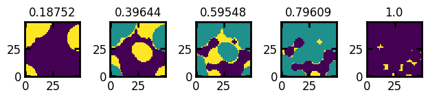
Note that extracting a slice at y=25 gives the same output as we have seen in the axis example above (default slice at mid-point axis):

fig, ax = ps.visualization.satn_to_panels(satn, im, bins=5, axis=1, slice=25)

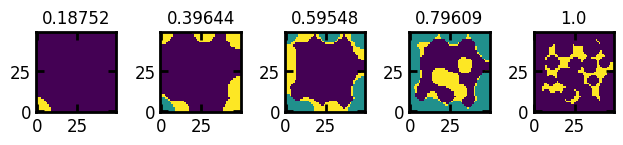
**kwargs

Additional keyword arguments can be sent to the imshow function, such as interpolation.

fig, ax = ps.visualization.satn_to_panels(
    satn, im, bins=5, axis=1, slice=25, interpolation=None
)