SNOW network extraction (advanced)#
The SNOW algorithm, published in Physical Review E, uses a marker-based watershed segmentation algorithm to partition an image into regions belonging to each pore. The main contribution of the SNOW algorithm is to find a suitable set of initial markers in the image so that the watershed is not over-segmented. SNOW is an acronym for Sub-Network of an Over-segmented Watershed. PoreSpy includes a predefined function called snow that applies all the steps automatically, but this example will illustrate the individual steps explicitly on a 3D image.
Start by importing the necessary packages:
import imageio
import matplotlib.pyplot as plt
import numpy as np
import openpnm as op
import scipy.ndimage as spim
from skimage.segmentation import watershed

import porespy as ps
from porespy.filters import find_peaks, trim_nearby_peaks, trim_saddle_points
from porespy.tools import randomize_colors

ps.settings.tqdm["disable"] = True
ps.visualization.set_mpl_style()
np.random.seed(10)
[04:04:09] WARNING PARDISO solver not installed on this platform. Simulations will be slow. _workspace.py:56
Generate artificial image#
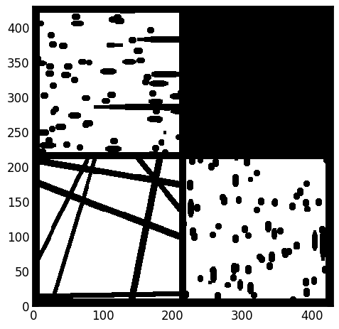
One of the main aims when developing the SNOW algorithm was to extract networks from images other than sandstone, which is the main material studied by geoscientists. For this demonstration we’ll use a high porosity (>85%) image of fibrous media.
im = ps.generators.cylinders(shape=[200, 200, 200], r=5, ncylinders=200)
fig, ax = plt.subplots()
ax.imshow(ps.visualization.show_planes(im), cmap=plt.cm.bone);
Step-by-step application of the SNOW algorithm#
Fist let’s find all the peaks of the distance transform which are theoretically suppose to lie at the center of each pore region. In reality this process finds too many peaks, but we’ll deal with this later.
sigma = 0.4
dt = spim.distance_transform_edt(input=im)
dt1 = spim.gaussian_filter(input=dt, sigma=sigma)
peaks = find_peaks(dt=dt)
The gaussian_filter is applied to the distance transform before finding the peaks, as this really reduces the number of spurious peaks by blurring the image slightly. The next few steps use custom made functions to help filter out remaining spurious peaks. The values of sigma and r are both adjustable but the defaults are usually acceptable.
print("Initial number of peaks: ", spim.label(peaks)[1])
peaks = trim_saddle_points(peaks=peaks, dt=dt1)
print("Peaks after trimming saddle points: ", spim.label(peaks)[1])
peaks = trim_nearby_peaks(peaks=peaks, dt=dt)
peaks, N = spim.label(peaks)
print("Peaks after trimming nearby peaks: ", N)
Initial number of peaks: 1167
Peaks after trimming saddle points: 568
Peaks after trimming nearby peaks: 410
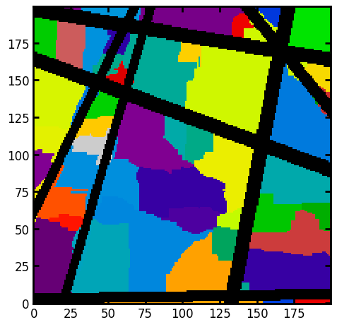
The final image processing step is to apply the marker-based watershed function that is available in scikit-image to partition the image into pores. This function is wrapped by the PoreSpy function partition_pore_space. watershed can be called directly, but remember to invert the distance transform so that peaks become valleys (just multiply by -1). This step is the slowest part of the process by far, but could be sped up if a faster implementation of watershed is used. The 300**3 image used in this example will take about 1 minute to complete.
regions = watershed(image=-dt, markers=peaks, mask=dt > 0)
regions = randomize_colors(regions)
This should produce an image with each voxel labelled according to which pore it belongs. The patches seem to be a bit odd looking but this is just an artifact of considering a 2D slice through a 3D image.
fig, ax = plt.subplots()
ax.imshow((regions * im)[:, :, 100], cmap=plt.cm.nipy_spectral);
Finally, this partitioned image can be passed to the network extraction function which analyzes the image and returns a Python dict containing the numerical properties of the network.
net = ps.networks.regions_to_network(regions * im, voxel_size=1)
This network can be opened in OpenPNM with ease, and then exported as a VTK file for viewing in ParaView.
pn = op.io.network_from_porespy(net)
You can inspect the network to see which properties have been extracted:
print(pn)
══════════════════════════════════════════════════════════════════════════════
net : <openpnm.network.Network at 0x7ff0ef30afd0>
――――――――――――――――――――――――――――――――――――――――――――――――――――――――――――――――――――――――――――――
  #  Properties                                                   Valid Values
――――――――――――――――――――――――――――――――――――――――――――――――――――――――――――――――――――――――――――――
  2  throat.conns                                                  1651 / 1651
  3  pore.coords                                                     410 / 410
  4  pore.region_label                                               410 / 410
  5  pore.phase                                                      410 / 410
  6  throat.phases                                                 1651 / 1651
  7  pore.region_volume                                              410 / 410
  8  pore.equivalent_diameter                                        410 / 410
  9  pore.local_peak                                                 410 / 410
 10  pore.global_peak                                                410 / 410
 11  pore.geometric_centroid                                         410 / 410
 12  throat.global_peak                                            1651 / 1651
 13  pore.inscribed_diameter                                         410 / 410
 14  pore.extended_diameter                                          410 / 410
 15  throat.inscribed_diameter                                     1651 / 1651
 16  throat.total_length                                           1651 / 1651
 17  throat.direct_length                                          1651 / 1651
 18  throat.perimeter                                              1651 / 1651
 19  pore.volume                                                     410 / 410
 20  pore.surface_area                                               410 / 410
 21  throat.cross_sectional_area                                   1651 / 1651
 22  throat.equivalent_diameter                                    1651 / 1651
――――――――――――――――――――――――――――――――――――――――――――――――――――――――――――――――――――――――――――――
  #  Labels                                                 Assigned Locations
――――――――――――――――――――――――――――――――――――――――――――――――――――――――――――――――――――――――――――――
  2  pore.all                                                              410
  3  throat.all                                                           1651
――――――――――――――――――――――――――――――――――――――――――――――――――――――――――――――――――――――――――――――
Overlaying the network and the image is requires using paraview since the image is in 3D. The is one gotcha due to the differences in how paraview and numpy number axes: it is necessary to rotate the image using ps.tools.align_image_with_openpnm:
im = ps.tools.align_image_with_openpnm(im)
imageio.volsave("image.tif", np.array(im, dtype=np.int8))
op.io.project_to_vtk(project=pn.project)