region_interface_areas

Calculate the interfacial area between all pairs of adjecent regions in a labeled image.

import matplotlib.pyplot as plt
import numpy as np
import porespy as ps
from skimage.morphology import disk
import inspect
inspect.signature(ps.metrics.region_interface_areas)

<Signature (regions, areas, voxel_size=1, strel=None)>

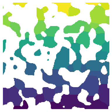
regions

The input image of the pore space partitioned into individual pore regions. Note that zeros in the image (solid phase) will not be considered for area calculation. Let’s create a test image:

np.random.seed(10)
im = ps.generators.blobs(shape=[200,200])
snow = ps.filters.snow_partitioning(im)
regions = snow.regions
fig, ax = plt.subplots(1, 1, figsize=[6, 6])
ax.imshow(regions/im, origin='lower', interpolation='none')
ax.axis(False);

areas

A list containing the areas of each regions, as determined by region_surface_area. Note that the region number and list index are offset by 1, such that the area for region 1 is stored in areas[0]. We must first calculate the areas of the regions in the test image, then given the regions and areas, we can calculate the interface areas of each neighbouring region. The region_interface_areas method returns a costum object containing the regions connections and interface area of each connection.

areas = ps.metrics.region_surface_areas(regions=regions)
conns, interface_areas = ps.metrics.region_interface_areas(regions, areas)
fig, ax = plt.subplots(1, 1, figsize=[6, 6])
ax.plot(np.arange(0,len(conns)), interface_areas, 'o')
plt.xlabel('interface (throat) number');
plt.ylabel('interface area (Voxel^2)');

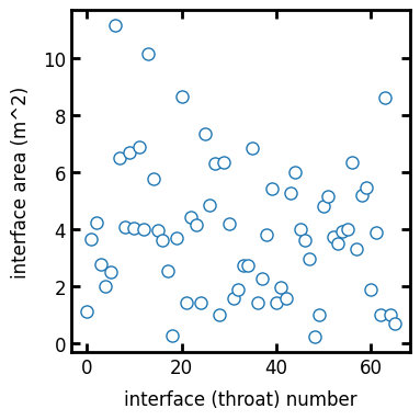
voxel_size

By default the voxel_size is 1. We can assign voxel size of the image as the input or apply the scaling on the results after the fact by multiplying the interface_areas to (voxel_size^2).

voxel_size=1e-1
conns, interface_areas = ps.metrics.region_interface_areas(regions, areas, voxel_size=voxel_size)
fig, ax = plt.subplots(1, 1, figsize=[6, 6])
ax.plot(np.arange(0,len(conns)), interface_areas, 'o')
plt.xlabel('interface (throat) number');
plt.ylabel('interface area (m^2)');

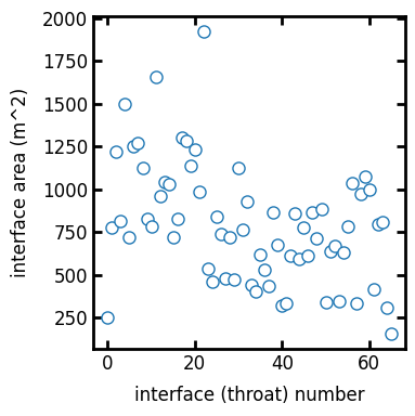
strel

By default the structuring element used to blur the region is a spherical element (or disk) with radius 1. This structuring element is used in the mesh_region method, which is called within the region_interface_areas function. The blur is perfomed using a simple convolution filter. The point is to create a greyscale region to allow the marching cubes algorithm (meshing algorithm) some freedom to conform the mesh to the surface. As the size of strel increases the region will become increasingly blurred and inaccurate.

voxel_size=1e-1
conns, interface_areas = ps.metrics.region_interface_areas(regions, areas, strel=disk(10))
fig, ax = plt.subplots(1, 1, figsize=[6, 6])
ax.plot(np.arange(0,len(conns)), interface_areas, 'o')
plt.xlabel('interface (throat) number');
plt.ylabel('interface area (m^2)');