pore_size_distribution

Calculates the pore size distribution in the image produced by either local thickness or porosimetry method where each voxel in the image shows the radius of the largest sphere (circle in 2D) that would overlap it.

import matplotlib.pyplot as plt
import numpy as np
import porespy as ps
import inspect
inspect.signature(ps.metrics.pore_size_distribution)

<Signature (im, bins=10, log=True, voxel_size=1)>

im

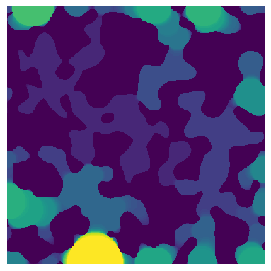
The input image csontaining the sizes of the largest sphere that overlaps each voxel. This image can be generated by implementing porosimetry or local_thickness filter on a binary image. Let’s generate a test image:

np.random.seed(10)
im = ps.generators.blobs(shape=[500, 500])
im = ps.filters.porosimetry(im)
fig, ax = plt.subplots(1, 1, figsize=[4, 4])
ax.imshow(im, origin='lower', interpolation='none')
ax.axis(False);

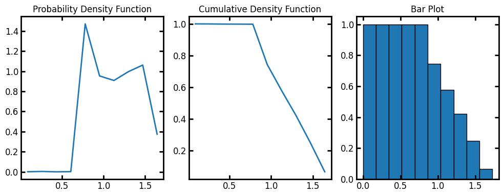
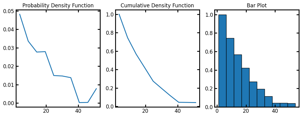
Now we can calculate the size distributions in the test image. pore_size_distribution returns a custom object with information of the distribution of the pore sizes. The x axis in the following images is the Log(pore radius).The histogram of logarithm (base-10) of pore sizes is useful to plot wide size distributions or to better visualize the data in the small size region.

data = ps.metrics.pore_size_distribution(im=im)
fig, ax = plt.subplots(1, 3, figsize=[10, 4])
ax[0].plot(data.bin_centers,data.pdf)
ax[1].plot(data.bin_centers,data.cdf)
ax[2].bar(data.bin_centers, data.cdf, data.bin_widths, edgecolor='k')
ax[0].set_title("Probability Density Function")
ax[1].set_title("Cumulative Density Function")
ax[2].set_title('Bar Plot');

bins

The default number of bins for the histogram is 10. Let’s increase the bins to 100:

data = ps.metrics.pore_size_distribution(im=im, bins=100)
fig, ax = plt.subplots(1, 3, figsize=[10, 4])
ax[0].plot(data.bin_centers,data.pdf)
ax[1].plot(data.bin_centers,data.cdf)
ax[2].bar(data.bin_centers, data.cdf, data.bin_widths, edgecolor='k')
ax[0].set_title("Probability Density Function")
ax[1].set_title("Cumulative Density Function")
ax[2].set_title('Bar Plot');

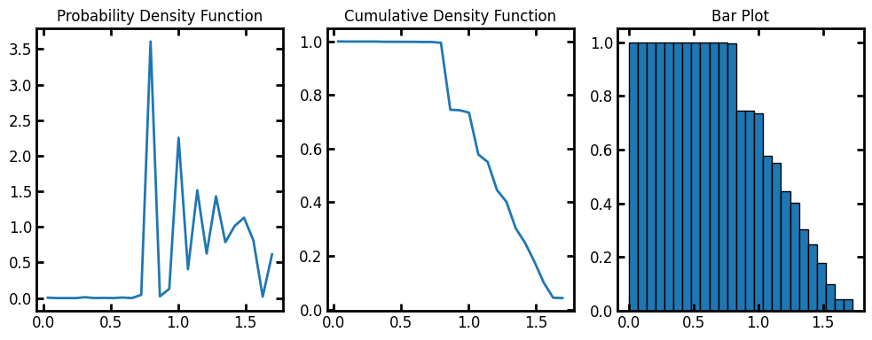
Plot results:

log

By default, the histogram binning is based on log(pore radius). We can calculate the size distribution base on pore radius with log=False. The resulting histogram binning is then performed on the pore radius values instead of log(pore radius. Note that for calculating the pore sizes base on diameter, bin_centers returned by pore_size_distribution must be multiplied by 2.

data = ps.metrics.pore_size_distribution(im=im, log=False)
fig, ax = plt.subplots(1, 3, figsize=[10, 4])
ax[0].plot(data.bin_centers,data.pdf)
ax[1].plot(data.bin_centers,data.cdf)
ax[2].bar(data.bin_centers, data.cdf, data.bin_widths, edgecolor='k')
ax[0].set_title("Probability Density Function")
ax[1].set_title("Cumulative Density Function")
ax[2].set_title('Bar Plot');

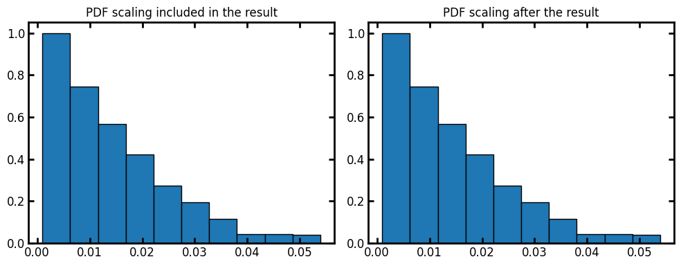
voxel_size

By default the voxel_size is 1. We can assign voxel size of the image as the input or apply the scaling on the results after the fact:

voxel_size=1e-3
data = ps.metrics.pore_size_distribution(im=im, voxel_size=voxel_size, log=False)
fig, ax = plt.subplots(1, 2, figsize=[10, 4])
ax[0].bar(data.bin_centers, data.cdf, data.bin_widths, edgecolor='k');
ax[0].set_title("PDF scaling included in the result");
data = ps.metrics.pore_size_distribution(im=im, log=False)
ax[1].bar(data.bin_centers*voxel_size, data.cdf, data.bin_widths*voxel_size, edgecolor='k');
ax[1].set_title("PDF scaling after the result");