rev_tortuosity

This notebook illustrates the use of rev_tortuosity, as well as the functionalities of the resulting object.

Import necessary packages

import matplotlib.pyplot as plt

import porespy as ps

ps.settings.loglevel = 50
ps.settings.tqdm['disable'] = False
ps.settings.tqdm['leave'] = True

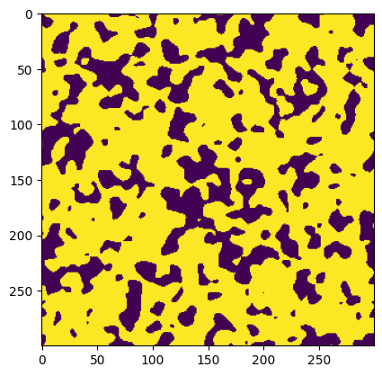
Generate an artificial 2D image for illustration purposes:

im = ps.generators.blobs([300]*2, porosity=0.7, blobiness=2, seed=1)
plt.imshow(im)

<matplotlib.image.AxesImage at 0x7f6b1fb79f10>

The function rev_tortuosity is able to accept slices for the subdomains to be processed. This can be generated using ps.tools.get_slices_random and ps.tools.get_slices_multigrid - previously ps.tools.subdivide. Alternatively, you can provide your own slice indices.

get_slices_random accepts an image, as well as the number of random slice indices to generate, this can be tweaked to suit your needs better.

get_slices_multigrid accepts an image, as well as the bounds for a range of slice sizes, and a step size, behaving similarly to np.arange.

slices = ps.tools.get_slices_random(im, 500)
rev = ps.metrics.rev_tortuosity(im, slices=slices, axis=0, dask_on=True)
converted = ps.tools.results_to_df(rev)

The results for the porosity profile are simultaneously obtained, and can be accessed with the various different attributes associated with the custom Results object.

print(rev)

――――――――――――――――――――――――――――――――――――――――――――――――――――――――――――――――――――――――――――――
Results of rev_tortuosity generated at Sat Jul 12 16:19:08 2025
――――――――――――――――――――――――――――――――――――――――――――――――――――――――――――――――――――――――――――――
porosity_orig             Dictionary with 500 items
porosity_perc             Dictionary with 500 items
g                         Dictionary with 500 items
tau                       Dictionary with 500 items
volume                    Dictionary with 500 items
length                    Dictionary with 500 items
axis                      Dictionary with 500 items
time                      Dictionary with 500 items
slice                     Dictionary with 500 items
――――――――――――――――――――――――――――――――――――――――――――――――――――――――――――――――――――――――――――――

Plotting the results

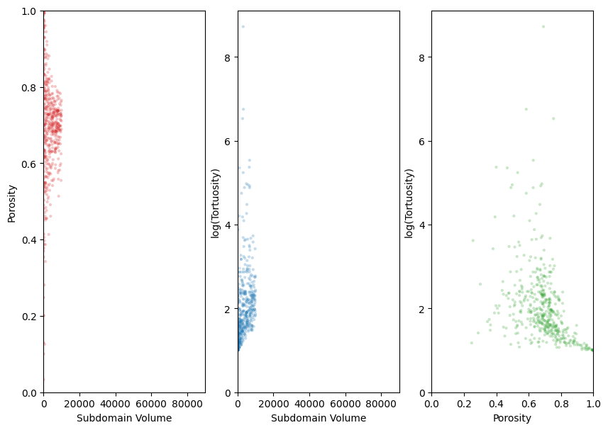
Lets plot the results and see if an REV has been found for both porosity and tortuosity. This would be roughly indicated by a stabilized value of porosity or tortuosity with an increasing subdomain volume.

fig, ax = plt.subplots(1, 3, figsize=[10, 7])
ax[0].scatter(rev.volume, rev.porosity_orig, marker='.', alpha=0.25, fc='tab:red', ec='none')
ax[1].scatter(rev.volume[rev.axis == 0], rev.tau[rev.axis == 0], marker='.', alpha=0.25, fc='tab:blue', ec='none')
ax[2].scatter(rev.porosity_perc[rev.axis == 0], rev.tau[rev.axis == 0], marker='.', alpha=0.25, fc='tab:green', ec='none')
ax[0].set_ylim([0, 1])
ax[0].set_xlim([0, im.size])
ax[0].set_ylabel('Porosity')
ax[0].set_xlabel('Subdomain Volume')
ax[1].set_ylim([0, None])
ax[1].set_xlim([0, im.size])
ax[1].set_ylabel('log(Tortuosity)')
ax[1].set_xlabel('Subdomain Volume')
ax[2].set_xlim([0, 1])
ax[2].set_ylim([0, None])
ax[2].set_xlabel('Porosity')
ax[2].set_ylabel('log(Tortuosity)')

Text(0, 0.5, 'log(Tortuosity)')

Alternatively, lets use get_slices_multigrid.

slices = ps.tools.get_slices_multigrid(im, [40, 300, 5])
rev = ps.metrics.rev_tortuosity(im, slices=slices, axis=0, dask_on=True)
converted = ps.tools.results_to_df(rev)

fig, ax = plt.subplots(1, 3, figsize=[10, 7])
ax[0].scatter(rev.volume, rev.porosity_orig, marker='.', alpha=0.25, fc='tab:red', ec='none')
ax[1].scatter(rev.volume[rev.axis == 0], rev.tau[rev.axis == 0], marker='.', alpha=0.25, fc='tab:blue', ec='none')
ax[2].scatter(rev.porosity_perc[rev.axis == 0], rev.tau[rev.axis == 0], marker='.', alpha=0.25, fc='tab:green', ec='none')
ax[0].set_ylim([0, 1])
ax[0].set_xlim([0, im.size])
ax[0].set_ylabel('Porosity')
ax[0].set_xlabel('Subdomain Volume')
ax[1].set_ylim([0, None])
ax[1].set_xlim([0, im.size])
ax[1].set_ylabel('log(Tortuosity)')
ax[1].set_xlabel('Subdomain Volume')
ax[2].set_xlim([0, 1])
ax[2].set_ylim([0, None])
ax[2].set_xlabel('Porosity')
ax[2].set_ylabel('log(Tortuosity)')

Text(0, 0.5, 'log(Tortuosity)')

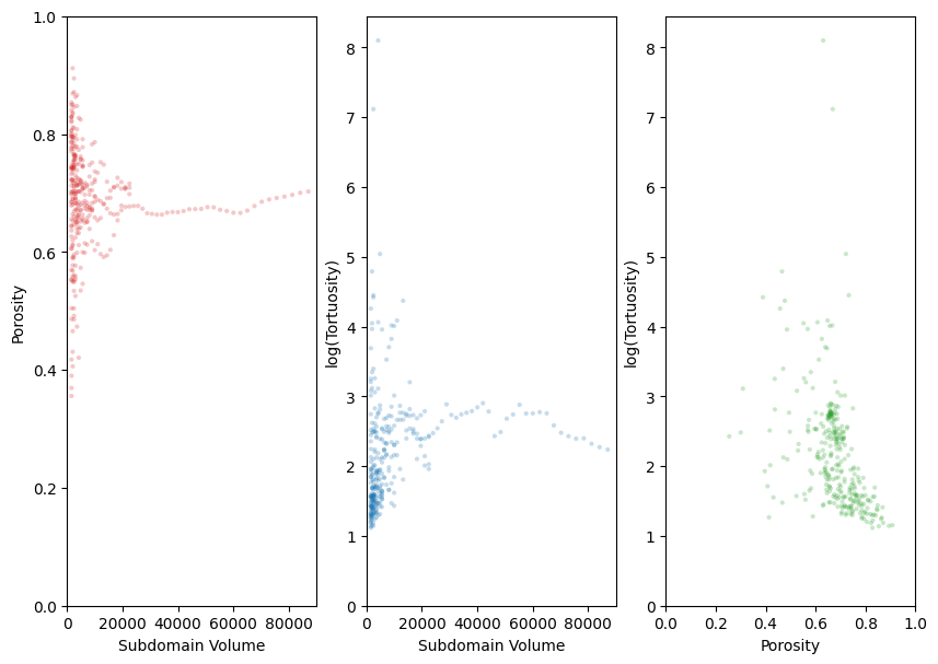
The multigrid method does not include overlap of blocks, so a block size which exceeds 50% of the image length will result in the remainder of the image being trimmed off, which can be seen in the first two graphs. This results in far less data points when compared to get_slices_random. The domain of the singular block being analyzed is being increased until it encompasses the whole image. The sudden drops in the tortuosity plot likely indicate the image “finding” an additional exit or percolating path from one face of the image to the opposite face.