WARNING Found non-percolating regions, were filled to percolate _dns.py:73
WARNING Found non-percolating regions, were filled to percolate _dns.py:73
WARNING Found non-percolating regions, were filled to percolate _dns.py:73
[03:59:29] WARNING Found non-percolating regions, were filled to percolate _dns.py:73
WARNING Found non-percolating regions, were filled to percolate _dns.py:73
WARNING Found non-percolating regions, were filled to percolate _dns.py:73
WARNING Found non-percolating regions, were filled to percolate _dns.py:73
WARNING Found non-percolating regions, were filled to percolate _dns.py:73
WARNING Found non-percolating regions, were filled to percolate _dns.py:73
WARNING Found non-percolating regions, were filled to percolate _dns.py:73
WARNING Found non-percolating regions, were filled to percolate _dns.py:73
WARNING Found non-percolating regions, were filled to percolate _dns.py:73
WARNING Found non-percolating regions, were filled to percolate _dns.py:73
[03:59:30] WARNING Found non-percolating regions, were filled to percolate _dns.py:73
WARNING Found non-percolating regions, were filled to percolate _dns.py:73
WARNING Found non-percolating regions, were filled to percolate _dns.py:73
WARNING Found non-percolating regions, were filled to percolate _dns.py:73
WARNING Found non-percolating regions, were filled to percolate _dns.py:73
WARNING Found non-percolating regions, were filled to percolate _dns.py:73
WARNING Found non-percolating regions, were filled to percolate _dns.py:73
WARNING Found non-percolating regions, were filled to percolate _dns.py:73
WARNING Found non-percolating regions, were filled to percolate _dns.py:73
WARNING Found non-percolating regions, were filled to percolate _dns.py:73
[03:59:31] WARNING Found non-percolating regions, were filled to percolate _dns.py:73
WARNING Found non-percolating regions, were filled to percolate _dns.py:73
WARNING Found non-percolating regions, were filled to percolate _dns.py:73
WARNING Found non-percolating regions, were filled to percolate _dns.py:73
WARNING Found non-percolating regions, were filled to percolate _dns.py:73
WARNING Found non-percolating regions, were filled to percolate _dns.py:73
WARNING Found non-percolating regions, were filled to percolate _dns.py:73
WARNING Found non-percolating regions, were filled to percolate _dns.py:73
WARNING Found non-percolating regions, were filled to percolate _dns.py:73
WARNING Found non-percolating regions, were filled to percolate _dns.py:73
WARNING Found non-percolating regions, were filled to percolate _dns.py:73
WARNING Found non-percolating regions, were filled to percolate _dns.py:73
[03:59:32] WARNING Found non-percolating regions, were filled to percolate _dns.py:73
WARNING Found non-percolating regions, were filled to percolate _dns.py:73
WARNING Found non-percolating regions, were filled to percolate _dns.py:73
WARNING Found non-percolating regions, were filled to percolate _dns.py:73
WARNING Found non-percolating regions, were filled to percolate _dns.py:73
WARNING Found non-percolating regions, were filled to percolate _dns.py:73
WARNING Found non-percolating regions, were filled to percolate _dns.py:73
WARNING Found non-percolating regions, were filled to percolate _dns.py:73
WARNING Found non-percolating regions, were filled to percolate _dns.py:73
WARNING Found non-percolating regions, were filled to percolate _dns.py:73
WARNING Found non-percolating regions, were filled to percolate _dns.py:73
WARNING Found non-percolating regions, were filled to percolate _dns.py:73
WARNING Found non-percolating regions, were filled to percolate _dns.py:73
[03:59:33] WARNING Found non-percolating regions, were filled to percolate _dns.py:73
WARNING Found non-percolating regions, were filled to percolate _dns.py:73
WARNING Found non-percolating regions, were filled to percolate _dns.py:73
WARNING Found non-percolating regions, were filled to percolate _dns.py:73
WARNING Found non-percolating regions, were filled to percolate _dns.py:73
WARNING Found non-percolating regions, were filled to percolate _dns.py:73
WARNING Found non-percolating regions, were filled to percolate _dns.py:73
WARNING Found non-percolating regions, were filled to percolate _dns.py:73
WARNING Found non-percolating regions, were filled to percolate _dns.py:73
WARNING Found non-percolating regions, were filled to percolate _dns.py:73
WARNING Found non-percolating regions, were filled to percolate _dns.py:73
WARNING Found non-percolating regions, were filled to percolate _dns.py:73
[03:59:34] WARNING Found non-percolating regions, were filled to percolate _dns.py:73
WARNING Found non-percolating regions, were filled to percolate _dns.py:73
WARNING Found non-percolating regions, were filled to percolate _dns.py:73
WARNING Found non-percolating regions, were filled to percolate _dns.py:73
WARNING Found non-percolating regions, were filled to percolate _dns.py:73
WARNING Found non-percolating regions, were filled to percolate _dns.py:73
WARNING Found non-percolating regions, were filled to percolate _dns.py:73
WARNING Found non-percolating regions, were filled to percolate _dns.py:73
WARNING Found non-percolating regions, were filled to percolate _dns.py:73
[03:59:35] WARNING Found non-percolating regions, were filled to percolate _dns.py:73
WARNING Found non-percolating regions, were filled to percolate _dns.py:73
WARNING Found non-percolating regions, were filled to percolate _dns.py:73
WARNING Found non-percolating regions, were filled to percolate _dns.py:73
WARNING Found non-percolating regions, were filled to percolate _dns.py:73
WARNING Found non-percolating regions, were filled to percolate _dns.py:73
WARNING Found non-percolating regions, were filled to percolate _dns.py:73
WARNING Found non-percolating regions, were filled to percolate _dns.py:73
[03:59:36] WARNING Found non-percolating regions, were filled to percolate _dns.py:73
WARNING Found non-percolating regions, were filled to percolate _dns.py:73
WARNING Found non-percolating regions, were filled to percolate _dns.py:73
WARNING Found non-percolating regions, were filled to percolate _dns.py:73
WARNING Found non-percolating regions, were filled to percolate _dns.py:73
WARNING Found non-percolating regions, were filled to percolate _dns.py:73
WARNING Found non-percolating regions, were filled to percolate _dns.py:73
WARNING Found non-percolating regions, were filled to percolate _dns.py:73
WARNING Found non-percolating regions, were filled to percolate _dns.py:73
WARNING Found non-percolating regions, were filled to percolate _dns.py:73
WARNING Found non-percolating regions, were filled to percolate _dns.py:73
WARNING Found non-percolating regions, were filled to percolate _dns.py:73
[03:59:37] WARNING Found non-percolating regions, were filled to percolate _dns.py:73
WARNING Found non-percolating regions, were filled to percolate _dns.py:73
WARNING Found non-percolating regions, were filled to percolate _dns.py:73
WARNING Found non-percolating regions, were filled to percolate _dns.py:73
WARNING Found non-percolating regions, were filled to percolate _dns.py:73
WARNING Found non-percolating regions, were filled to percolate _dns.py:73
WARNING Found non-percolating regions, were filled to percolate _dns.py:73
WARNING Found non-percolating regions, were filled to percolate _dns.py:73
WARNING Found non-percolating regions, were filled to percolate _dns.py:73
WARNING Found non-percolating regions, were filled to percolate _dns.py:73
WARNING Found non-percolating regions, were filled to percolate _dns.py:73
[03:59:38] WARNING Found non-percolating regions, were filled to percolate _dns.py:73
WARNING Found non-percolating regions, were filled to percolate _dns.py:73
WARNING Found non-percolating regions, were filled to percolate _dns.py:73
WARNING Found non-percolating regions, were filled to percolate _dns.py:73
WARNING Found non-percolating regions, were filled to percolate _dns.py:73
WARNING Found non-percolating regions, were filled to percolate _dns.py:73
WARNING Found non-percolating regions, were filled to percolate _dns.py:73
WARNING Found non-percolating regions, were filled to percolate _dns.py:73
WARNING Found non-percolating regions, were filled to percolate _dns.py:73
WARNING Found non-percolating regions, were filled to percolate _dns.py:73
WARNING Found non-percolating regions, were filled to percolate _dns.py:73
WARNING Found non-percolating regions, were filled to percolate _dns.py:73
WARNING Found non-percolating regions, were filled to percolate _dns.py:73
WARNING Found non-percolating regions, were filled to percolate _dns.py:73
[03:59:39] WARNING Found non-percolating regions, were filled to percolate _dns.py:73
WARNING Found non-percolating regions, were filled to percolate _dns.py:73
WARNING Found non-percolating regions, were filled to percolate _dns.py:73
WARNING Found non-percolating regions, were filled to percolate _dns.py:73
WARNING Found non-percolating regions, were filled to percolate _dns.py:73
WARNING Found non-percolating regions, were filled to percolate _dns.py:73
WARNING Found non-percolating regions, were filled to percolate _dns.py:73
WARNING Found non-percolating regions, were filled to percolate _dns.py:73
WARNING Found non-percolating regions, were filled to percolate _dns.py:73
WARNING Found non-percolating regions, were filled to percolate _dns.py:73
WARNING Found non-percolating regions, were filled to percolate _dns.py:73
[03:59:40] WARNING Found non-percolating regions, were filled to percolate _dns.py:73
WARNING Found non-percolating regions, were filled to percolate _dns.py:73
WARNING Found non-percolating regions, were filled to percolate _dns.py:73
WARNING Found non-percolating regions, were filled to percolate _dns.py:73
WARNING Found non-percolating regions, were filled to percolate _dns.py:73
WARNING Found non-percolating regions, were filled to percolate _dns.py:73
WARNING Found non-percolating regions, were filled to percolate _dns.py:73
WARNING Found non-percolating regions, were filled to percolate _dns.py:73
WARNING Found non-percolating regions, were filled to percolate _dns.py:73
[03:59:41] WARNING Found non-percolating regions, were filled to percolate _dns.py:73
WARNING Found non-percolating regions, were filled to percolate _dns.py:73
WARNING Found non-percolating regions, were filled to percolate _dns.py:73
WARNING Found non-percolating regions, were filled to percolate _dns.py:73
WARNING Found non-percolating regions, were filled to percolate _dns.py:73
WARNING Found non-percolating regions, were filled to percolate _dns.py:73
WARNING Found non-percolating regions, were filled to percolate _dns.py:73
WARNING Found non-percolating regions, were filled to percolate _dns.py:73
WARNING Found non-percolating regions, were filled to percolate _dns.py:73
WARNING Found non-percolating regions, were filled to percolate _dns.py:73
WARNING Found non-percolating regions, were filled to percolate _dns.py:73
[03:59:42] WARNING Found non-percolating regions, were filled to percolate _dns.py:73
WARNING Found non-percolating regions, were filled to percolate _dns.py:73
WARNING Found non-percolating regions, were filled to percolate _dns.py:73
WARNING Found non-percolating regions, were filled to percolate _dns.py:73
WARNING Found non-percolating regions, were filled to percolate _dns.py:73
WARNING Found non-percolating regions, were filled to percolate _dns.py:73
WARNING Found non-percolating regions, were filled to percolate _dns.py:73
WARNING Found non-percolating regions, were filled to percolate _dns.py:73
WARNING Found non-percolating regions, were filled to percolate _dns.py:73
WARNING Found non-percolating regions, were filled to percolate _dns.py:73
WARNING Found non-percolating regions, were filled to percolate _dns.py:73
WARNING Found non-percolating regions, were filled to percolate _dns.py:73
[03:59:43] WARNING Found non-percolating regions, were filled to percolate _dns.py:73
WARNING Found non-percolating regions, were filled to percolate _dns.py:73
WARNING Found non-percolating regions, were filled to percolate _dns.py:73
WARNING Found non-percolating regions, were filled to percolate _dns.py:73
WARNING Found non-percolating regions, were filled to percolate _dns.py:73
WARNING Found non-percolating regions, were filled to percolate _dns.py:73
WARNING Found non-percolating regions, were filled to percolate _dns.py:73
WARNING Found non-percolating regions, were filled to percolate _dns.py:73
WARNING Found non-percolating regions, were filled to percolate _dns.py:73
WARNING Found non-percolating regions, were filled to percolate _dns.py:73
WARNING Found non-percolating regions, were filled to percolate _dns.py:73
WARNING Found non-percolating regions, were filled to percolate _dns.py:73
WARNING Found non-percolating regions, were filled to percolate _dns.py:73
WARNING Found non-percolating regions, were filled to percolate _dns.py:73
WARNING Found non-percolating regions, were filled to percolate _dns.py:73
WARNING Found non-percolating regions, were filled to percolate _dns.py:73
WARNING Found non-percolating regions, were filled to percolate _dns.py:73
WARNING Found non-percolating regions, were filled to percolate _dns.py:73
WARNING Found non-percolating regions, were filled to percolate _dns.py:73
WARNING Found non-percolating regions, were filled to percolate _dns.py:73
[03:59:44] WARNING Found non-percolating regions, were filled to percolate _dns.py:73
WARNING Found non-percolating regions, were filled to percolate _dns.py:73
WARNING Found non-percolating regions, were filled to percolate _dns.py:73
WARNING Found non-percolating regions, were filled to percolate _dns.py:73
WARNING Found non-percolating regions, were filled to percolate _dns.py:73
WARNING Found non-percolating regions, were filled to percolate _dns.py:73
WARNING Found non-percolating regions, were filled to percolate _dns.py:73
WARNING Found non-percolating regions, were filled to percolate _dns.py:73
WARNING Found non-percolating regions, were filled to percolate _dns.py:73
WARNING Found non-percolating regions, were filled to percolate _dns.py:73
WARNING Found non-percolating regions, were filled to percolate _dns.py:73
WARNING Found non-percolating regions, were filled to percolate _dns.py:73
WARNING Found non-percolating regions, were filled to percolate _dns.py:73
[03:59:45] WARNING Found non-percolating regions, were filled to percolate _dns.py:73
WARNING Found non-percolating regions, were filled to percolate _dns.py:73
WARNING Found non-percolating regions, were filled to percolate _dns.py:73
WARNING Found non-percolating regions, were filled to percolate _dns.py:73
WARNING Found non-percolating regions, were filled to percolate _dns.py:73
WARNING Found non-percolating regions, were filled to percolate _dns.py:73
WARNING Found non-percolating regions, were filled to percolate _dns.py:73
WARNING Found non-percolating regions, were filled to percolate _dns.py:73
WARNING Found non-percolating regions, were filled to percolate _dns.py:73
WARNING Found non-percolating regions, were filled to percolate _dns.py:73
WARNING Found non-percolating regions, were filled to percolate _dns.py:73
WARNING Found non-percolating regions, were filled to percolate _dns.py:73
WARNING Found non-percolating regions, were filled to percolate _dns.py:73
WARNING Found non-percolating regions, were filled to percolate _dns.py:73
[03:59:46] WARNING Found non-percolating regions, were filled to percolate _dns.py:73
WARNING Found non-percolating regions, were filled to percolate _dns.py:73
WARNING Found non-percolating regions, were filled to percolate _dns.py:73
WARNING Found non-percolating regions, were filled to percolate _dns.py:73
WARNING Found non-percolating regions, were filled to percolate _dns.py:73
――――――――――――――――――――――――――――――――――――――――――――――――――――――――――――――――――――――――――――――
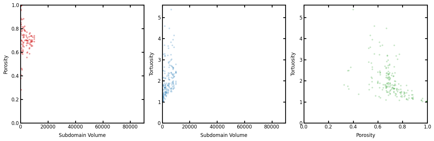
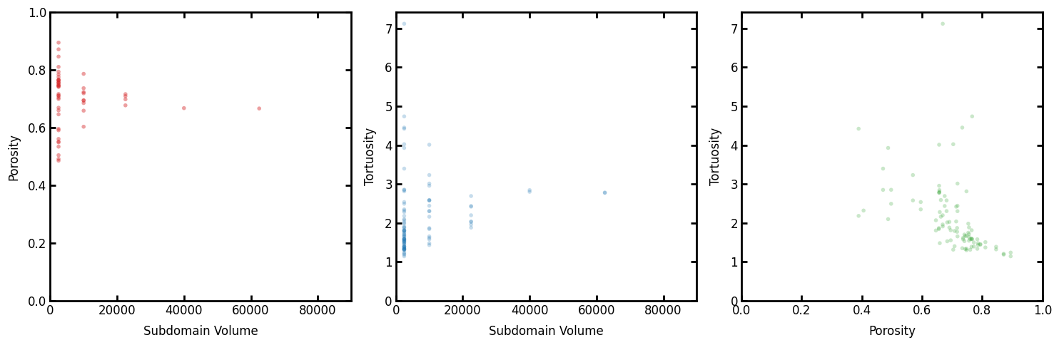
Results of rev_tortuosity generated at Sun Mar 1 03:59:46 2026
――――――――――――――――――――――――――――――――――――――――――――――――――――――――――――――――――――――――――――――
porosity_orig Dictionary with 400 items
porosity_perc Dictionary with 400 items
g Dictionary with 400 items
tau Dictionary with 400 items
volume Dictionary with 400 items
length Dictionary with 400 items
axis Dictionary with 400 items
time Dictionary with 400 items
slice Dictionary with 400 items
――――――――――――――――――――――――――――――――――――――――――――――――――――――――――――――――――――――――――――――