Opening and Preparing Images

The examples in the generators section have numerous examples on how to generate artificial images, but ultimately most people will be working with real images obtained from X-ray tomography or serial sectioning. This tutorial will cover a few different aspects about how to open these images for using a Jupyter notebook, or a Python workflow in general.

Let’s import the packages and functions that we’ll be needing:

import imageio.v2 as imageio
import porespy as ps
import numpy as np
from skimage.io import imread_collection
from matplotlib.pyplot import subplots

[17:44:26] ERROR    PARDISO solver not installed, run `pip install pypardiso`. Otherwise,          _workspace.py:56
                    simulations will be slow. Apple M chips not supported.                                         

Opening a Folder of 2D tif Images

Using ImageJ

ImageJ is the ultimate image processing tool kit. It has many functions and filters for doing quantitative analysis, usually added via plug-ins (see note below), but it’s also very good at converting between file types and formats.

If you have a folder full of 2D images which are either microscope images obtained by serial sectioning or reconstructions of backprojections from X-ray tomography, then you’ll want to convert these into a single tif image. tif supports 3D images, so all the individual 2D images can be stacked together into a single file.

This can be done in ImageJ using “File/Import/Image Sequence” as shown in the screenshots below. Note that the images must be named with a numerical value indicating its order in the sequence, like “slice_001.tif”.

A dialog box will appear asking you about some of the details, which are usually correct by default:

Finally, you’ll want to save this new 3d tif image, which can be done with “save as”:

ImageJ and Fiji

ImageJ has a plugin architecture to add functionality. At some point it was realized that most users install numerous plugins, so Fiji was created, which is ImageJ with a large selection of the most popular plugins preinstalled. The name Fiji is actually a recursive acronym for “Fiji Is Just ImageJ”

Directly in Python

If you’d rather not get manually involved, then it’s also possible to do this in Python. The scikit-image package comes with a handy funciton for just this purpose. It only takes a few minutes to get used to how it works:

seq = imread_collection("../../docs/_static/images/Sample 1/*.tif")

Now let’s inspect the result. We can see a list of files loaded in the files attribute:

seq.files

[]

And we can access the loaded images from the seq object as if it were a list:

fig, ax = subplots(figsize=[5, 5])
ax.imshow(seq[0]);

---------------------------------------------------------------------------
IndexError                                Traceback (most recent call last)
Cell In[4], line 2
      1 fig, ax = subplots(figsize=[5, 5])
----> 2 ax.imshow(seq[0]);

File /opt/hostedtoolcache/Python/3.10.14/x64/lib/python3.10/site-packages/skimage/io/collection.py:301, in ImageCollection.__getitem__(self, n)
    298     raise TypeError('slicing must be with an int or slice object')
    300 if type(n) is int:
--> 301     n = self._check_imgnum(n)
    302     idx = n % len(self.data)
    304     if ((self.conserve_memory and n != self._cached) or
    305             (self.data[idx] is None)):

File /opt/hostedtoolcache/Python/3.10.14/x64/lib/python3.10/site-packages/skimage/io/collection.py:357, in ImageCollection._check_imgnum(self, n)
    355     n = n % num
    356 else:
--> 357     raise IndexError(f"There are only {num} images in the collection")
    358 return n

IndexError: There are only 0 images in the collection

We can convert this list into a 3D image as follows:

im3d = np.zeros([*seq[0].shape, len(seq)])
for i, im in enumerate(seq):
    im3d[..., i] = im

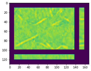
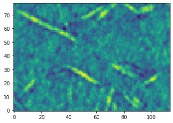
And now we can use porespy to visualize it:

fig, ax = subplots(figsize=[5, 5])
ax.imshow(ps.visualization.show_planes(im3d));

Convert to Binary

In this tutorial we will not do anything to clean or denoise these images, as that deserves it’s own tutorial. Here we’ll just apply a threshold to convert a boolean with True indicating solid (the fibers above) and False indicating void.

First we need to look at the range of values in the image:

fig, ax = subplots(figsize=[5, 5])
ax.hist(im3d.flatten(), bins=25, edgecolor='k');

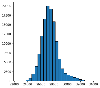
From the above histogram we can see that the values span from 22000 to 34000. We can just search for a value which does a decent job of segmenting the solid and void by trial and error:

fig, ax = subplots(figsize=[5, 5])
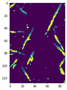
ax.imshow(im3d[..., 0] < 30000);

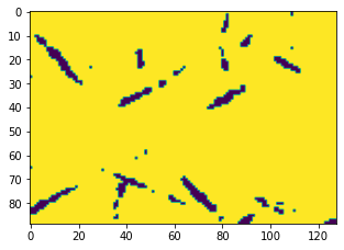
Because the image is noisy the result is not perfect. But let’s apply this threshold to the entire image now, then visualize the 3D stack:

im = im3d < 30000
fig, ax = subplots(figsize=[5, 5])
ax.imshow(ps.visualization.sem(im, axis=2));

Opening a 3D Stack

Assuming that the 2D images have been turned into a 3D image, as described above, it is straightforward to load them:

im2 = imageio.volread('../../docs/_static/images/Sample 1.tif')
ps.imshow(im2, axis=0);

Saving a 3D Image

Once you have created a nice image that you want to save, perhaps for visualization in Paraview, you can also use the imageio package:

imageio.volsave('my image.tif', np.array(im, dtype=np.int8))