pc_curve

This single method can convert either (a) images containing invasion size or (b) invasion pressure results, such as those produced by porosimetry and drainage, respectively.

import porespy as ps
import numpy as np
import matplotlib.pyplot as plt

[19:54:50] ERROR    PARDISO solver not installed, run `pip install pypardiso`. Otherwise,          _workspace.py:56
                    simulations will be slow. Apple M chips not supported.                                         

No module named 'pyedt'

Generate an image and apply the drainage function:

np.random.seed(0)
im = ps.generators.blobs(shape=[200, 200], porosity=0.6)
pc = ps.filters.capillary_transform(im, sigma=0.01, theta=180, voxel_size=1e-5)
drn = ps.simulations.drainage(im)

pc

The function can accept an image of invasion pressures, such as that produced by drainage or qbip:

pc_curve = ps.metrics.pc_curve(im=im, pc=drn.im_pc)

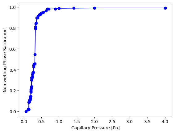
The function returns an object with pc and snwp as attributes which can be plotted directly:

plt.plot(pc_curve.pc, pc_curve.snwp, 'b-o')
plt.xlabel('Capillary Pressure [Pa]')
plt.ylabel('Non-wetting Phase Saturation');

Alternatively, if the size map is available but not the capillary pressure map, then size_to_pc can be used first:

pc = ps.filters.size_to_pc(im=im, size=drn.im_size, sigma=0.01, theta=180, voxel_size=1e-5)
data = ps.metrics.pc_curve(im=im, pc=pc)

Matplotlib can be used to plot the curve:

plt.plot(data.pc, data.snwp, 'r-o')
plt.xlabel('Capillary Pressure [Pa]')
plt.ylabel('Non-wetting Phase Saturation');